Machine Learning - Neural Networks Representation Part I

This series of articles are the study notes of " Machine Learning ", by Prof. Andrew Ng., Stanford University. This article is the notes of week 4, Neural Networks Representation Part I. It contains topics about nonlinear hypotheses, neurons and the brain, model representation.  

Neural Networks Representation Part I

In this and in the next set of sections, I'd like to tell you about a learning algorithm called a Neural Network. We're going to first talk about the representation and then in the next set of videos talk about learning algorithms for it. 

The neural network will be able to represent complex models that form non-linear hypotheses.

Neutral networks is actually a pretty old idea, but had fallen out of favor for a while. But today, it is the state of the art technique for many different machine learning problems. So why do we need yet another learning algorithm? We already have linear regression and we have logistic regression, so why do we need, you know, neural networks? In order to motivate the discussion of neural networks, let me start by showing you a few examples of machine learning problems where we need to learn complex non-linear hypotheses.

1. Non-linear hypotheses

Example 1: Classification problem

Consider a supervised learning classification problem where  you have a training set like this. If you want to apply logistic regression to  this problem, one thing you could do is apply logistic regression with a lot of  nonlinear features like that. So here, g as usual is the sigmoid function, and  we can include lots of polynomial terms like these. And, if you include enough  polynomial terms then, you know, maybe you can get a hypotheses that separates  the positive and negative examples.

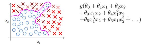
This particular method works well when you have only, say, two features x₁ and x₂ because you can then include all those polynomial terms of x₁ and  x₂. But for many interesting machine learning problems would have a lot more features than just two.

Second order: n²/2 = 5000 features

We've been talking for a while about housing prediction, and suppose you have a housing classification problem rather than a regression problem, like maybe if you have different features of a house, and you want to predict what are the odds that your house will be sold within the next six months, so that will be a classification problem. And as we saw we can come up with quite a lot of features, maybe a hundred different features of different houses. For a problem like this, if you were to include all the quadratic terms, all of these, even all of the quadratic that is the second or the polynomial terms, there would be a lot of them. There would be terms  like x ₁ squared, x ₁ x ₂, x ₁ x ₃, you know, x ₁ x ₄ up to x ₁ x ₁₀₀ and then you have  x ₂ squared, x ₂ x ₃ and so on. And  if you include just the second order terms, that is, the terms that are a product of two of these terms x ₁ times x ₁ and soon, then, for the case of n equals 100, you end up with about 5000 features. And, asymptotically, then umber of quadratic features grows roughly as order n squared, where n is the number of the original features, like x ₁ through x ₁₀₀ that we had.

And its actually closer to n²/2. So including all the quadratic features doesn't seem like it's maybe a good idea, because  that is a lot of features and you might up overfitting the training set, and it can also be computationally expensive.

Third order: O(n³) ≈ 170000 features

So 5000 features seems like a lot, if you were to include the cubic, or third order known of each others, the  x₁, x₂, x₃. You know, x₁ squared,x₂, x₁₀ and x₁₁, x₁₇ and so on. You can imaging there are gonna be a lot of these features. In fact, they are going to be order and cube such features and if any is 100 you can compute that, you end up with on the order of about 170,000 such cubic features and so including these higher auto-polynomial features when your original feature set end is large this really dramatically blows up your feature space and this doesn't seem like a good way to come up with additional features with which to build none many classifiers when n is large.

Example 2: Computer vision

For many machine learning problems, n will be pretty large. Here's an example. Let's consider the problem of computer vision. 

And suppose you want to use machine learning to train a classifier to examine an image and tell us whether or not the image is a car. Many people wonder why computer vision could be difficult. I mean when you and I look at this picture it is so obvious what this is. You wonder how is it that a learning algorithm could possibly fail to know what this picture is. To understand why computer vision is hard let's zoom into a small part of the image like that area where the little red rectangle is.

It turns out that where you and I see a car, the computer sees that. What it sees is this matrix, or this grid, of pixel intensity values that tells us the brightness of each pixel in the image. So the computer vision problem is to look at this matrix of pixel intensity values, and tell us that these numbers represent the door handle of a car.

Concretely, when we use machine learning to build a car detector, what we do is we come up with a label training set, with, let's say, a few label examples of cars and a few label examples of things that are not cars, then we give our training set to the learning algorithm trained a classifier and then, you know, we may test it and show the new image and ask, "What is this new thing?".

To understand why we need nonlinear hypotheses, let's take a look at some of the images of cars and maybe non-cars that we might feed to our learning algorithm. Let's pick a couple of pixel locations in our images, so that's pixel one location and pixel two location, and let's plot this car, you know, at the location, at a certain point, depending on the intensities of pixel one and pixel two. And let's do this with a few other images. So let's take a different example of the car and you know, look at the same two pixel locations and that image has a different intensity for pixel one and a different intensity for pixel two.

So, it ends up at a different location on the figure. And then let's plot some negative examples as well. That's a non-car, that's a non-car. And if we do this for more and more examples using the pluses to denote cars and minuses to denote non-cars, what we'll find is that the cars and non-cars end up lying in different regions of the space, and what we need therefore is some sort of non-linear hypotheses to try to separate out the two classes.

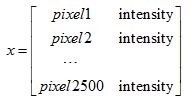
50×50 gray scale image=2500 features

What is the dimension of the feature space? Suppose we were to use just  50 by 50 pixel images. Now that suppose our images were pretty small ones, just 50 pixels on the side. Then we would  have 2500 pixels, and so the dimension of our feature size will be n = 2500 where our feature vector x is a list of all the pixel testings, the pixel brightness of pixel one, the brightness of pixel two, and so on down to the pixel brightness of the last pixel where, you know, in a typical computer representation, each of these may be values between say 0 to 255 if it gives us the gray scale value. So we have n equals 2500, and that's if we were using gray scale images.

50×50 RGB image=7500 features

If we were using RGB images with separate red, green and blue values, we would have n = 7500. 

Nonlinear hypothesis  including quadratic features = 3,000,000 features

So, if we were to try to learn a nonlinear hypothesis by including all the quadratic features, that is all the terms of the form, Xi times Xj, while with the 2500 pixels we would end up with a total of 3 million features. And that's just too large to be reasonable; the computation would be very expensive to find and to represent all of these three million features per training example.

Quaduatic features (): x_i × x_j ≈3 million features

So, simple logistic regression together with adding in maybe the quadratic or the cubic features - that's just not a good way to learn complex nonlinear hypotheses when n is large because you just end up with too many features.

2. Neurons and the brain

Neural Networks are a pretty old algorithm that was originally motivated by the goal of having machines that can mimic the brain. Now in this class, of course I'm teaching Neural Networks to you because they work really well for different machine learning problems.

In this section, I'd like to give you some of the background on Neural Networks. So that we can get a sense of what we can expect them to do. Both in the sense of applying them to modern day machine learning problems, as well as for those of you that might be interested in maybe the big AI dream of someday building truly intelligent machines.

History of Neural Networks

• Origins: Algorithms that try to mimic the brain.
• Was very widely used in 80s and early 90s; popularity diminished in late 90s.
• Recent resurgence: State-of-the-art technique for many applications

More recently, Neural Networks  have had a major recent resurgence. One of the reasons for this resurgence is that Neural Networks are computationally some what more expensive algorithm and so, it was only, you know, maybe somewhat more recently that computers became fast enough to really run large scale Neural Networks and because of that as well as a few other technical reasons which we'll talk about later, modern Neural Networks today are the state of the art technique for many applications.

The “one learning algorithm” hypothesis 

The brain can learn to see process images than to hear, learn to process our sense of touch. We can, you know, learn to do math, learn to do calculus, and the brain does so many different and amazing things.

the way the brain does it is worth just a single learning algorithm. This is just a hypothesis but let me share with you some of the evidence for this.

Re-wire: auditory cortex will learn to see

This part of the brain, that little red part of the brain, is your auditory cortex and the way you're understanding my voice now is your ear is taking the sound signal and routing the sound signal to your auditory cortex and that's what's allowing you to understand my words.

Neuroscientists have done the following fascinating experiments where you cut the wire from the ears to the auditory cortex and you re-wire,in this case an animal's brain, so that the signal from the eyes to the optic nerve eventually gets routed to the auditory cortex. If you do this it turns out, the auditory cortex will learn to see. And this is in every single sense of the word see as we know it.

Re-wire: omatosensory cortex will learn to see

Here's another example. That red piece of brain tissue is your somatosensory cortex. That's how you process your sense of touch. If you do a similar re-wiring process then the somatosensory cortex will learn to see.

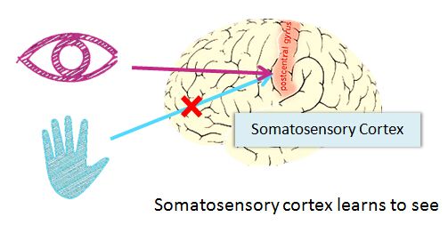
Same piece of physical brain tissue can process sight or sound or touch

Because of this and other similar experiments, these are called neuro-rewiring experiments. There's this sense that if the same piece of physical brain tissue can process sight or sound or touch then maybe there is one learning algorithm that can process sight or sound or touch. And instead of needing to implement a thousand different programs or a thousand different algorithms to do, the thousand wonderful things that the brain does, maybe what we need to do is figure out some approximation or to whatever the brain's learning algorithm is and implement that and that the brain learned by itself how to process these different types of data.

So, it's pretty amazing to what extent is as if you can plug in almost any sensor to the brain and the brain's learning algorithm will just figure out how to learn from that data and deal with that data.

3. Model representation I 

In this video, I want to start telling you about how we represent neural networks. In other words,

how we represent our hypothesis or how we represent our model when using neural networks. Neural networks were developed as simulating neurons or networks of neurons in the brain. So, to explain the hypothesis representation let's start by looking at what a single neuron in the brain looks like.

Neuron in the brain 

Your brain and mine is jam packed full of neurons like these and neurons are cells in the brain. And two things to draw attention to. 

Dendrites : input wires

The neuron has a cell body, and moreover, the neuron has a number of input wires, and these are called the dendrites. You think of them as input wires, and these receive inputs from other locations. 

Axon: output wire

And a neuron also has an output wire called an Axon, and this output wire is what it uses to send signals to other neurons, so to send messages to other neurons.

So, at a simplistic level what a neuron is, is a computational unit that gets a number of inputs through it input wires and does some computation and then it says outputs via its axon to other nodes or to other neurons in the brain.

Neuron model: Logistic unit

Sigmoid (logistic) activation function:

We call θ the parameters or the weights.

To explain these specific computations represented by a neural network, here's a little bit more notation.

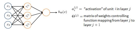
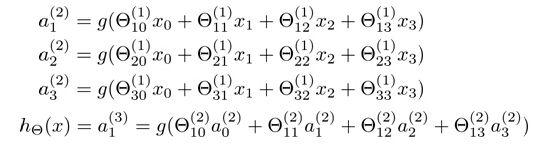
So here are the computations that are represented by this diagram. This first hidden unit here has it's value computed as follows:

There's a is a₁⁽²⁾ is equal to the sigmoid function of the sigmoid activation function, also called the logistics activation function, apply to this sort of linear combination of these inputs. And then this second hidden unit has this activation value computer as sigmoid of this. And similarly for this third hidden unit is computed by that formula.

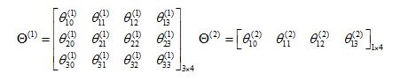
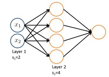
If network has s_j units in layerj ,s_j+1 units in layer j +1, then θ^(j) will be the dimension of s_j+1×(s_j+1). 

Example:

what is the dimension of θ⁽¹⁾?

s₁=2, s₂=4,dimension of θ⁽¹⁾=s₂×(s₁+1) = 4 × 3

To summarize, what we've done is shown how a picture like this over here defines an artificial neural network which defines a function h that maps with x's input values to hopefully to some space that provisions y. And these hypothesis are parameterized by parameters denoting with a capital theta so that, as we vary theta, we get different hypothesis and we get different functions.  Mapping say from x to y. So this gives us a mathematical definition of how to represent the hypothesis in the neural network.