lstm原文_LSTM:《Long Short-Term Memory》的翻译并解读
LSTM:《Long Short-Term Memory》的翻译并解读
目录
Long Short-Term Memory
Abstract
1 INTRODUCTION
2 PREVIOUS WORK
3 CONSTANT ERROR BACKPROP
3.1 EXPONENTIALLY DECAYING ERROR
3.2 CONSTANT ERROR FLOW: NAIVE APPROACH
4 LONG SHORT-TERM MEMORY
5 EXPERIMENTS
5.1 EXPERIMENT 1: EMBEDDED REBER GRAMMAR
Long Short-Term Memory
论文原文地址01:https://arxiv.org/pdf/1506.04214.pdf地址02:https://www.bioinf.jku.at/publications/older/2604.pdf
Abstract
Learning to store information over extended time intervals via recurrent backpropagation takes a very long time, mostly due to insucient, decaying error back ow. We brie y review Hochreiter's 1991 analysis of this problem, then address it by introducing a novel, ecient, gradient-based method called Long Short-Term Memory" (LSTM). Truncating the gradient where this does not do harm, LSTM can learn to bridge minimal time lags in excess of 1000 discrete time steps by enforcing constant error ow through constant error carrousels" within special units. Multiplicative gate units learn to open and close access to the constant error ow. LSTM is local in space and time; its computational complexity per time step and weight is O(1). Our experiments with arti cial data involve local, distributed, real-valued, and noisy pattern representations. In comparisons with RTRL, BPTT, Recurrent Cascade-Correlation, Elman nets, and Neural Sequence Chunking, LSTM leads to many more successful runs, and learns much faster. LSTM also solves complex, arti cial long time lag tasks that have never been solved by previous recurrent network algorithms.通过周期性的反向传播学习,在扩展的时间间隔内存储信息需要很长的时间,这主要是由于不确定的、衰减的错误导致的。我们简要回顾了Hochreiter在1991年对这个问题的分析,然后介绍了一种新颖的、独特的、基于梯度的方法,称为LSTM (LSTM)。在不造成伤害的情况下截断梯度,LSTM可以学习在超过1000个离散时间步长的最小时间滞后上桥接,方法是通过在特殊单元内的“恒定误差轮盘”强制执行恒定误差。乘性门单元学习打开和关闭访问的恒定误差低。LSTM在空间和时间上都是局部的;其每时间步长的计算复杂度和权值为O(1)。我们对人工数据的实验包括局部的、分布式的、实值的和有噪声的模式表示。在与RTRL、BPTT、周期性级联相关、Elman网和神经序列分块的比较中,LSTM带来了更多的成功运行,并且学习速度更快。LSTM还解决了以前的递归网络算法所不能解决的复杂、人工的长时间滞后问题。
1 INTRODUCTION
Recurrent networks can in principle use their feedback connections to store representations of recent input events in form of activations (short-term memory", as opposed to long-term memory" embodied by slowly changing weights). This is potentially signicant for many applications, including speech processing, non-Markovian control, and music composition (e.g., Mozer 1992). The most widely used algorithms for learning what to put in short-term memory, however, take too much time or do not work well at all, especially when minimal time lags between inputs and corresponding teacher signals are long. Although theoretically fascinating, existing methods do not provide clear practical advantages over, say, backprop in feedforward nets with limited time windows. This paper will review an analysis of the problem and suggest a remedy.
递归网络原则上可以使用它们的反馈连接以激活的形式存储最近输入事件的表示(“短期记忆”,而不是“长期记忆”,后者由缓慢变化的权重表示)。这对许多应用程序都有潜在的重要性,包括语音处理、非马尔可夫控制和音乐作曲(例如,Mozer 1992)。然而,最广泛使用的学习短期记忆的算法要么花费了太多时间,要么根本就不能很好地工作,尤其是在输入和相应教师信号之间的最小时滞很长时。虽然理论上很吸引人,但现有的方法并没有提供明显的实际优势,例如,在有限时间窗口的前馈网络中,backprop。本文将对这一问题进行分析,并提出解决办法。The problem. With conventional Back-Propagation Through Time" (BPTT, e.g., Williams and Zipser 1992, Werbos 1988) or Real-Time Recurrent Learning" (RTRL, e.g., Robinson and Fallside 1987), error signals owing backwards in time" tend to either (1) blow up or (2) vanish: the temporal evolution of the backpropagated error exponentially depends on the size of the weights (Hochreiter 1991). Case (1) may lead to oscillating weights, while in case (2) learning to bridge long time lags takes a prohibitive amount of time, or does not work at all (see section 3). 这个问题。与传统反向传播通过时间”(BPTT,例如,1992年威廉姆斯和拉链,Werbos 1988)或实时复发性学习”(RTRL,例如,罗宾逊和Fallside 1987),误差信号在时间上向后由于”倾向于(1)炸毁或(2):消失的时间演化backpropagated误差指数的大小取决于重量(Hochreiter 1991)。情形(1)可能会导致权值的振荡,而情形(2)学习如何桥接长时间滞后的情况会花费大量的时间,或者根本不起作用(参见第3节)。The remedy. This paper presents Long Short-Term Memory" (LSTM), a novel recurrent network architecture in conjunction with an appropriate gradient-based learning algorithm. LSTM is designed to overcome these error back- ow problems. It can learn to bridge time intervals in excess of 1000 steps even in case of noisy, incompressible input sequences, without loss of short time lag capabilities. This is achieved by an ecient, gradient-based algorithm for an architecture enforcing constant (thus neither exploding nor vanishing) error ow through internal states of special units (provided the gradient computation is truncated at certain architecture-specic points | this does not aect long-term error ow though). 补救措施。本文提出了一种新的递归网络结构——长短时记忆(LSTM),并结合适当的梯度学习算法。LSTM的设计就是为了克服这些错误的反向问题。它可以学习桥接超过1000步的时间间隔,即使在有噪声、不可压缩的输入序列的情况下,也不会损失短时间延迟能力。这是通过一种特殊的、基于梯度的算法来实现的,它针对的是一种通过特殊单元的内部状态来执行常量(因此既不会爆炸也不会消失)的错误(假设梯度计算在某些特定的体系结构点|被截断,但这并不影响长期的错误)。Outline of paper. Section 2 will brie y review previous work. Section 3 begins with an outline of the detailed analysis of vanishing errors due to Hochreiter (1991). It will then introduce a naive approach to constant error backprop for didactic purposes, and highlight its problems concerning information storage and retrieval. These problems will lead to the LSTM architecture as described in Section 4. Section 5 will present numerous experiments and comparisons with competing methods. LSTM outperforms them, and also learns to solve complex, articial tasks no other recurrent net algorithm has solved. Section 6 will discuss LSTM's limitations and advantages. The appendix contains a detailed description of the algorithm (A.1), and explicit error ow formulae (A.2).第二部分将简要回顾以前的工作。第3节以详细分析Hochreiter(1991)所造成的消失误差的大纲开始。然后,它将介绍一种用于教学目的的幼稚的不断错误支持方法,并突出其在信息存储和检索方面的问题。这些问题将导致第4节中描述的LSTM体系结构。第5节将提供大量的实验和与竞争方法的比较。LSTM比它们做得更好,而且还学会了解决复杂的人工任务,这是其他递归网络算法所不能解决的。第6节将讨论LSTM的局限性和优点。附录中有算法的详细描述(a .1),以及公式的显式误差(a .2)。
2 PREVIOUS WORK
This section will focus on recurrent nets with time-varying inputs (as opposed to nets with stationary inputs and xpoint-based gradient calculations, e.g., Almeida 1987, Pineda 1987).
本节将集中讨论具有时变输入的递归网络(而不是具有固定输入和基于x点的梯度计算的网络,例如Almeida 1987和Pineda 1987)。
Gradient-descent variants. The approaches of Elman (1988), Fahlman (1991), Williams (1989), Schmidhuber (1992a), Pearlmutter (1989), and many of the related algorithms in Pearlmutter's comprehensive overview (1995) suer from the same problems as BPTT and RTRL (see Sections 1 and 3).
梯度下降法变体。Elman(1988)、Fahlman(1991)、Williams(1989)、Schmidhuber (1992a)、Pearlmutter(1989)的方法,以及Pearlmutter的综合综述(1995)中的许多相关算法,都是从与BPTT和RTRL相同的问题中提出的(见第1节和第3节)
Time-delays. Other methods that seem practical for short time lags only are Time-Delay Neural Networks (Lang et al. 1990) and Plate's method (Plate 1993), which updates unit activations based on a weighted sum of old activations (see also de Vries and Principe 1991). Lin et al. (1995) propose variants of time-delay networks called NARX networks.
时间延迟。其他似乎只适用于短时间滞后的方法有时滞神经网络(Lang et al. 1990)和Plate法(Plate 1993),后者基于旧激活的加权和更新单位激活(参见de Vries和Principe 1991)。Lin等人(1995)提出了时延网络的变体NARX网络。
Time constants. To deal with long time lags, Mozer (1992) uses time constants in uencing changes of unit activations (deVries and Principe's above-mentioned approach (1991) may in fact be viewed as a mixture of TDNN and time constants). For long time lags, however, the time constants need external ne tuning (Mozer 1992). Sun et al.'s alternative approach (1993) updates the activation of a recurrent unit by adding the old activation and the (scaled) current net input. The net input, however, tends to perturb the stored information, which makes long-term storage impractical.
时间常量。为了处理长时间滞后,Mozer(1992)使用时间常数来表示单位激活的变化(deVries and Principe’s上述方法(1991)实际上可以看作是TDNN和时间常数的混合物)。然而,对于长时间滞后,时间常数需要外部ne调谐(Mozer 1992)。Sun等人的替代方法(1993)通过添加旧的激活和(缩放的)当前净输入来更新一个经常性单元的激活。然而,净输入往往会干扰所存储的信息,这使得长期存储变得不切实际。
Ring's approach. Ring (1993) also proposed a method for bridging long time lags. Whenever a unit in his network receives con icting error signals, he adds a higher order unit in uencing appropriate connections. Although his approach can sometimes be extremely fast, to bridge a time lag involving 100 steps may require the addition of 100 units. Also, Ring's net does not generalize to unseen lag durations.
环的方法。Ring(1993)也提出了一种桥接长时间滞后的方法。当他的网络中的一个单元接收到通信错误信号时,他就增加一个更高阶的单元来建立适当的连接。虽然他的方法有时非常快,但要跨越100步的时间延迟可能需要增加100个单元。同样,环网也不能推广到看不见的滞后时间。
Bengio et al.'s approaches. Bengio et al. (1994) investigate methods such as simulated annealing, multi-grid random search, time-weighted pseudo-Newton optimization, and discrete error propagation. Their latch" and 2-sequence" problems are very similar to problem 3a with minimal time lag 100 (see Experiment 3). Bengio and Frasconi (1994) also propose an EM approach for propagating targets. With n so-called state networks", at a given time, their system can be in one of only n dierent states. See also beginning of Section 5. But to solve continuous problems such as the adding problem" (Section 5.4), their system would require an unacceptable number of states (i.e., state networks).
Bengio等人的方法。Bengio等人(1994)研究了模拟退火、多网格随机搜索、时间加权伪牛顿优化和离散误差传播等方法。他们的“闩锁”和“2-序列”问题与3a问题非常相似,只有最小的滞后时间100(见实验3)。Bengio和Frasconi(1994)也提出了一种EM方法来传播目标。对于n个所谓的“状态网络”,在给定的时间内,它们的系统只能处于n种不同状态中的一种。参见第5节的开头。但是,为了解决诸如“添加问题”(第5.4节)之类的连续问题,它们的系统将需要不可接受的状态数(即状态的网络)。
Kalman lters. Puskorius and Feldkamp (1994) use Kalman lter techniques to improve recurrent net performance. Since they use a derivative discount factor imposed to decay exponentially the eects of past dynamic derivatives," there is no reason to believe that their Kalman Filter Trained Recurrent Networks will be useful for very long minimal time lags. Second order nets. We will see that LSTM uses multiplicative units (MUs) to protect error ow from unwanted perturbations. It is not the rst recurrent net method using MUs though. For instance, Watrous and Kuhn (1992) use MUs in second order nets. Some dierences to LSTM are:
- (1) Watrous and Kuhn's architecture does not enforce constant error ow and is not designed to solve long time lag problems.
- (2) It has fully connected second-order sigma-pi units, while the LSTM architecture's MUs are used only to gate access to constant error ow.
- (3) Watrous and Kuhn's algorithm costs O(W2 ) operations per time step, ours only O(W), where W is the number of weights. See also Miller and Giles (1993) for additional work on MUs.
- Kalman lters. Puskorius and Feldkamp (1994)使用Kalman lter技术来提高经常性净绩效。由于他们使用一个衍生品折扣因子来指数衰减过去动态衍生品的影响,“我们没有理由相信他们的卡尔曼滤波训练的递归网络在很长一段时间内都是有用的。”二阶网络。我们将看到LSTM使用乘法单位(MUs)来保护错误不受不必要的干扰。但它不是第一个使用MUs的递归网络方法。例如,Watrous和Kuhn(1992)在二阶网中使用MUs。LSTM的一些不同之处是:(1)Watrous和Kuhn的架构不强制恒定的错误,也不是为了解决长时间滞后的问题而设计的。
- (2)它具有完全连通的二阶sigma-pi单元,而LSTM体系结构的MUs仅用于对恒定误差低的门访问。
- (3) Watrous和Kuhn的算法每时间步需要O(W2)个操作,我们的算法只需要O(W)个操作,其中W是权值的个数。有关MUs的其他工作也见Miller和Giles(1993)。
Simple weight guessing. To avoid long time lag problems of gradient-based approaches we may simply randomly initialize all network weights until the resulting net happens to classify all training sequences correctly. In fact, recently we discovered (Schmidhuber and Hochreiter 1996, Hochreiter and Schmidhuber 1996, 1997) that simple weight guessing solves many of the problems in (Bengio 1994, Bengio and Frasconi 1994, Miller and Giles 1993, Lin et al. 1995) faster than the algorithms proposed therein. This does not mean that weight guessing is a good algorithm. It just means that the problems are very simple. More realistic tasks require either many free parameters (e.g., input weights) or high weight precision (e.g., for continuous-valued parameters), such that guessing becomes completely infeasible.
简单的猜测。为了避免基于梯度的方法的长时间滞后问题,我们可以简单地随机初始化所有网络权值,直到最终得到的网络正确地对所有训练序列进行分类。事实上,最近我们发现(Schmidhuber and Hochreiter 1996, Hochreiter and Schmidhuber 1996, 1997)简单的重量猜测解决了(Bengio 1994, Bengio and Frasconi 1994, Miller and Giles 1993, Lin et al. 1995)中的许多问题,比其中提出的算法更快。这并不意味着猜测权重是一个好的算法。这意味着问题很简单。更实际的任务需要许多自由参数(例如,输入权值)或较高的权值精度(例如,连续值参数),这样猜测就变得完全不可行的。
Adaptive sequence chunkers. Schmidhuber's hierarchical chunker systems (1992b, 1993) do have a capability to bridge arbitrary time lags, but only if there is local predictability across the subsequences causing the time lags (see also Mozer 1992). For instance, in his postdoctoral thesis (1993), Schmidhuber uses hierarchical recurrent nets to rapidly solve certain grammar learning tasks involving minimal time lags in excess of 1000 steps. The performance of chunker systems, however, deteriorates as the noise level increases and the input sequences become less compressible. LSTM does not suer from this problem.自适应序列chunkers。Schmidhuber的分层chunker系统(1992b, 1993)确实具有桥接任意时间滞后的能力,但前提是子序列具有局部可预测性,从而导致时间滞后(参见Mozer 1992)。例如,在他的博士后论文(1993)中,Schmidhuber使用层次递归网络来快速解决某些语法学习任务,这些任务涉及的时间延迟最小,超过了1000步。然而,随着噪声水平的提高和输入序列的可压缩性的降低,chunker系统的性能会下降。LSTM不能解决这个问题。
3 CONSTANT ERROR BACKPROP 固定误差支持
3.1 EXPONENTIALLY DECAYING ERROR 指数衰减误差
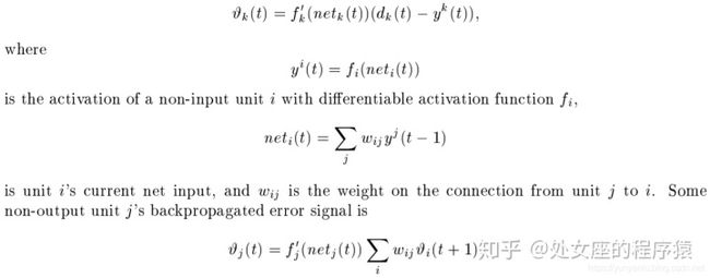
Conventional BPTT (e.g. Williams and Zipser 1992). Output unit k's target at time t is denoted by dk (t). Using mean squared error, k's error signal is
传统的BPTT(如Williams和Zipser 1992)。输出单元k在t时刻的目标用dk (t)表示,利用均方误差,k的误差信号为
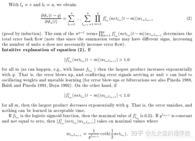
The corresponding contribution to wjl 's total weight update is #j (t)yl (t 1), where is the learning rate, and l stands for an arbitrary unit connected to unit j. Outline of Hochreiter's analysis (1991, page 19-21). Suppose we have a fully connected net whose non-input unit indices range from 1 to n. Let us focus on local error ow from unit u to unit v (later we will see that the analysis immediately extends to global error ow). The error occurring at an arbitrary unit u at time step t is propagated back into time" for q time steps, to an arbitrary unit v. This will scale the error by the following fact
wjl的总权重更新的相应贡献是#j (t)yl (t 1),其中为学习率,l表示连接到j单元的任意单元。Hochreiter分析概要(1991年,第19-21页)。假设我们有一个完全连通的网络,它的非输入单位指数范围从1到n。让我们关注从单位u到单位v的局部误差ow(稍后我们将看到分析立即扩展到全局误差ow)。发生在任意单位u上的时间步长t的误差被传播回时间中,对于q时间步长,传播回任意单位v
3.2 CONSTANT ERROR FLOW: NAIVE APPROACH 常量错误流:简单的方法
A single unit. To avoid vanishing error signals, how can we achieve constant error ow through a single unit j with a single connection to itself? According to the rules above, at time t, j's local error back ow is #j (t) = f 0 j (netj (t))#j (t + 1)wjj . To enforce constant error ow through j, we h j, we
一个单元。为了避免消失的错误信号,我们如何通过一个单一的单位j与一个单一的连接到自己实现恒定的错误低?根据上面的规则,在t时刻,j的本地错误返回ow是#j (t) = f0 j (netj (t))#j (t + 1)wjj。为了通过j来执行常误差ow,我们h j,我们
In the experiments, this will be ensured by using the identity function fj : fj (x) = x; 8x, and by setting wjj = 1:0. We refer to this as the constant error carrousel (CEC). CEC will be LSTM's central feature (see Section 4). Of course unit j will not only be connected to itself but also to other units. This invokes two obvious, related problems (also inherent in all other gradient-based approaches):在实验中,利用恒等函数fj: fj (x) = x来保证;设置wjj = 1:0。我们称之为常误差卡鲁塞尔(CEC)。CEC将是LSTM的中心特性(参见第4节)。当然,单元j不仅与自身相连,还与其他单元相连。这引发了两个明显的、相关的问题(也是所有其他基于梯度的方法所固有的):
- 1. Input weight con ict: for simplicity, let us focus on a single additional input weight wji . Assume that the total error can be reduced by switching on unit j in response to a certain input, and keeping it active for a long time (until it helps to compute a desired output). Provided i is nonzero, since the same incoming weight has to be used for both storing certain inputs and ignoring others, wji will often receive con icting weight update signals during this time (recall that j is linear): these signals will attempt to make wji participate in (1) storing the input (by switching on j) and (2) protecting the input (by preventing j from being switched o by irrelevant later inputs). This con ict makes learning dicult, and calls for a more context-sensitive mechanism for controlling write operations" through input weights.
- 2. Output weight con ict: assume j is switched on and currently stores some previous input. For simplicity, let us focus on a single additional outgoing weight wkj . The same wkj has to be used for both retrieving j's content at certain times and preventing j from disturbing k at other times. As long as unit j is non-zero, wkj will attract con icting weight update signals generated during sequence processing: these signals will attempt to make wkj participate in (1) accessing the information stored in j and | at dierent times | (2) protecting unit k from being perturbed by j. For instance, with many tasks there are certain short time lag errors" that can be reduced in early training stages. However, at later training stages j may suddenly start to cause avoidable errors in situations that already seemed under control by attempting to participate in reducing more dicult long time lag errors". Again, this con ict makes learning dicult, and calls for a more context-sensitive mechanism for controlling read operations" through output weights.
- 1. 输入权值约束:为了简单起见,我们将重点放在单个额外的输入权值wji上。假设可以通过打开单元j来响应某个输入,并长时间保持它处于活动状态(直到它有助于计算所需的输出),从而减少总错误。提供我是零,因为相同的传入的重量必须是用于存储特定的输入和无视他人,wji通常会接收con ict重量更新信号在此期间(回想一下,j是线性):这些信号将试图使wji参与(1)存储输入(通过打开j)和(2)保护输入(通过阻止j被无关紧要了o后输入)。这使得学习变得困难,需要一种更上下文敏感的机制来“通过输入权重”控制写操作。
- 2. 输出权值:假设j已经打开,并且当前存储了一些以前的输入。为了简单起见,让我们关注单个额外的输出权wkj。相同的wkj必须在特定时间用于检索j的内容,在其他时间用于防止j干扰k。只要单位j是零,wkj将吸引con ict重量更新信号生成的序列处理期间:这些信号将试图使wkj参与(1)访问的信息存储在j和| | dierent倍(2)保护单元凯西从被摄动j。例如,许多任务有些短时间延迟错误”,可以减少在早期训练阶段。然而,在后来的训练阶段,j可能会突然开始在那些似乎已经在控制之中的情况下,通过尝试减少更多的长时间延迟错误来造成可避免的错误。同样,这一缺点使学习变得困难,需要一种更上下文敏感的机制来“通过输出权重”控制读操作。
Of course, input and output weight con icts are not specic for long time lags, but occur for short time lags as well. Their eects, however, become particularly pronounced in the long time lag case: as the time lag increases, (1) stored information must be protected against perturbation for longer and longer periods, and | especially in advanced stages of learning | (2) more and more already correct outputs also require protection against perturbation.
Due to the problems above the naive approach does not work well except in case of certain simple problems involving local input/output representations and non-repeating input patterns (see Hochreiter 1991 and Silva et al. 1996). The next section shows how to do it right.当然,输入和输出的权系数在长时间滞后时是不特定的,但在短时间滞后时也会出现。除,然而,在长时间滞后的情况下尤为明显:随着时间间隔的增加,(1)存储信息必须防止扰动时间却越来越长,学习|和|尤其是晚期(2)越来越多的正确输出也需要防止扰动。
由于上述问题,天真的方法不能很好地工作,除非某些简单的问题涉及本地输入/输出表示和非重复输入模式(见Hochreiter 1991和Silva et al. 1996)。下一节将展示如何正确地执行此操作。
4 LONG SHORT-TERM MEMORY
Memory cells and gate units. To construct an architecture that allows for constant error ow through special, self-connected units without the disadvantages of the naive approach, we extend the constant error carrousel CEC embodied by the self-connected, linear unit j from Section 3.2 by introducing additional features. A multiplicative input gate unit is introduced to protect the memory contents stored in j from perturbation by irrelevant inputs. Likewise, a multiplicative output gate unit is introduced which protects other units from perturbation by currently irrelevant memory contents stored in j.记忆单元和门单元。为了构建一个允许通过特殊的、自连接的单元实现恒定误差的体系结构,同时又不存在朴素方法的缺点,我们通过引入额外的特性来扩展3.2节中自连接的线性单元j所包含的恒定误差carrousel CEC。为了保护存储在j中的存储内容不受无关输入的干扰,引入了乘法输入门单元。同样地,一个乘法输出门单元被引入,它保护其他单元不受当前不相关的存储在j中的内存内容的干扰。
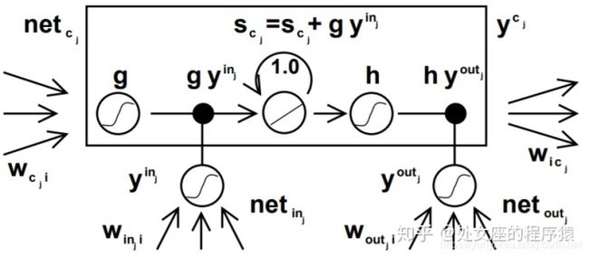
net Figure 1: Architecture of memory cel l cj (the box) and its gate units inj ; outj . The self-recurrent connection (with weight 1.0) indicates feedback with a delay of 1 time step. It builds the basis of the constant error carrousel" CEC. The gate units open and close access to CEC. See text and appendix A.1 for details.
图1:memory cel l cj(盒子)的结构和它的门单元inj;outj。自循环连接(权值为1.0)表示反馈延迟1个时间步长。它建立了恒定误差carrousel“CEC”的基础。星门单元打开和关闭CEC的入口。详情见正文和附录A.1。
ls. Why gate units? To avoid input weight con icts, inj controls the error ow to memory cell cj 's input connections wcj i . To circumvent cj 's output weight con icts, outj controls the error ow from unit j's output connections. In other words, the net can use inj to decide when to keep or override information in memory cell cj , and outj to decide when to access memory cell cj and when to prevent other units from being perturbed by cj (see Figure 1).
为什么门单位?为了避免输入权值冲突,inj控制了内存单元cj的输入连接的误差。为了绕过cj的输出权值,outj控制来自单位j的输出连接的错误。换句话说,网络可以使用inj来决定何时在内存单元cj中保留或覆盖信息,而使用outj来决定何时访问内存单元cj以及何时防止其他单元受到cj的干扰(参见图1)。
Error signals trapped within a memory cell's CEC cannot change { but dierent error signals owing into the cell (at dierent times) via its output gate may get superimposed. The output gate will have to learn which errors to trap in its CEC, by appropriately scaling them. The input gate will have to learn when to release errors, again by appropriately scaling them. Essentially, the multiplicative gate units open and close access to constant error ow through CEC.
存储单元的CEC中的错误信号不能改变{但是通过输出门进入单元的不同错误信号(在不同的时间)可以被叠加。通过适当地扩展,输出门必须了解在其CEC中应该捕获哪些错误。输入门必须学会何时释放错误,再次通过适当地扩展它们。从本质上说,乘性门单元通过CEC打开和关闭对恒定误差的访问。
Distributed output representations typically do require output gates. Not always are both gate types necessary, though | one may be sucient. For instance, in Experiments 2a and 2b in Section 5, it will be possible to use input gates only. In fact, output gates are not required in case of local output encoding | preventing memory cells from perturbing already learned outputs can be done by simply setting the corresponding weights to zero. Even in this case, however, output gates can be benecial: they prevent the net's attempts at storing long time lag memories (which are usually hard to learn) from perturbing activations representing easily learnable short time lag memories. (This will prove quite useful in Experiment 1, for instance.)
分布式输出表示通常需要输出门。虽然|一个可能是必需的,但两个门不一定都是必需的。例如,在第5节的2a和2b实验中,将可能只使用输入门。事实上,在本地输出编码为|的情况下,不需要输出门,只要将相应的权值设置为0,就可以防止内存单元干扰已经学习过的输出。然而,即使在这种情况下,输出门也可能是有益的:它们阻止了网络存储长时间滞后记忆(通常很难学习)的尝试,从而干扰了代表容易学习的短时间滞后记忆的激活。(例如,这在实验1中将被证明非常有用。)
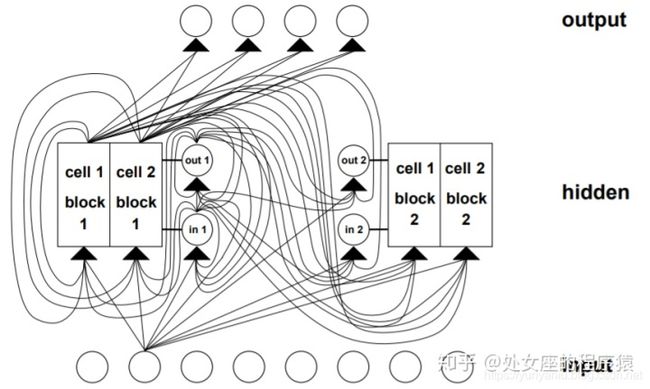
Network topology. We use networks with one input layer, one hidden layer, and one output layer. The (fully) self-connected hidden layer contains memory cells and corresponding gate units (for convenience, we refer to both memory cells and gate units as being located in the hidden layer). The hidden layer may also contain conventional" hidden units providing inputs to gate units and memory cells. All units (except for gate units) in all layers have directed connections (serve as inputs) to all units in the layer above (or to all higher layers { Experiments 2a and 2b).
Memory cell blocks. S memory cells sharing the same input gate and the same output gate form a structure called a memory cell block of size S". Memory cell blocks facilitate information storage | as with conventional neural nets, it is not so easy to code a distributed input within a single cell. Since each memory cell block has as many gate units as a single memory cell (namely two), the block architecture can be even slightly more ecient (see paragraph computational complexity"). A memory cell block of size 1 is just a simple memory cell. In the experiments (Section 5), we will use memory cell blocks of various sizes.
网络拓扑结构。我们使用一个输入层、一个隐含层和一个输出层的网络。(完全)自连接的隐层包含内存单元和相应的栅极单元(为了方便起见,我们将位于隐层中的内存单元和栅极单元都称为隐层)。所述隐层还可以包含提供栅极单元和存储器单元输入的常规“隐单元”。所有层中的所有单元(门单元除外)都有指向连接(作为输入)到上面层中的所有单元(或所有更高的层{实验2a和2b)。
存储单元块。共享相同的输入门和输出门的内存单元形成一个称为大小为S的内存单元块的结构。记忆单元块促进信息存储|与传统的神经网络一样,在单个单元内编码分布式输入并不容易。由于每个内存单元块与单个内存单元(即两个)具有同样多的门单元,因此块架构甚至可以更特殊一些(请参阅段落“计算复杂性”)。大小为1的内存单元块只是一个简单的内存单元。在实验(第5部分)中,我们将使用不同大小的存储单元块。
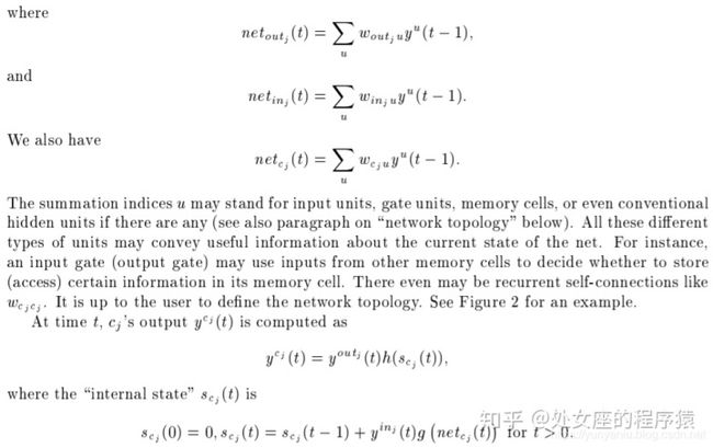
Learning. We use a variant of RTRL (e.g., Robinson and Fallside 1987) which properly takes into account the altered, multiplicative dynamics caused by input and output gates. However, to ensure non-decaying error backprop through internal states of memory cells, as with truncated BPTT (e.g., Williams and Peng 1990), errors arriving at memory cell net inputs" (for cell cj , this includes netcj , netinj , netoutj ) do not get propagated back further in time (although they do serve to change the incoming weights). Only within2 memory cells, errors are propagated back through previous internal states scj . To visualize this: once an error signal arrives at a memory cell output, it gets scaled by output gate activation and h0 . Then it is within the memory cell's CEC, where it can ow back indenitely without ever being scaled. Only when it leaves the memory cell through the input gate and g, it is scaled once more by input gate activation and g 0 . It then serves to change the incoming weights before it is truncated (see appendix for explicit formulae).
Computational complexity. As with Mozer's focused recurrent backprop algorithm (Mozer 1989), only the derivatives @scj @wil need to be stored and updated. Hence the LSTM algorithm is very ecient, with an excellent update complexity of O(W), where W the number of weights (see details in appendix A.1). Hence, LSTM and BPTT for fully recurrent nets have the same update complexity per time step (while RTRL's is much worse). Unlike full BPTT, however, LSTM is local in space and time3 : there is no need to store activation values observed during sequence processing in a stack with potentially unlimited size.
学习。我们使用RTRL的一个变体(例如,Robinson和Fallside 1987),它适当地考虑了输入和输出门所引起的变化的乘法动力学。然而,以确保non-decaying错误backprop通过内部状态的记忆细胞,与截断BPTT(例如,威廉姆斯和彭1990),错误到达存储单元网络输入”(细胞cj,这包括netcj、netinj netoutj)得不到传播更久远的时代(尽管他们服务变化的权重)。只有在2个内存单元中,错误才会通过之前的内部状态scj传播回来。为了可视化这一点:一旦一个错误信号到达一个内存单元输出,它将被输出门激活和h0缩放。然后它在记忆细胞的CEC中,在那里它可以无限地慢下来而不需要被缩放。只有当它通过输入门和g离开存储单元时,它才通过输入门激活和g 0再次被缩放。然后,它用于在截断之前更改传入的权重(有关显式公式,请参阅附录)。
计算的复杂性。与Mozer的重点循环支持算法(Mozer 1989)一样,只需要存储和更新导数@scj @wil。因此LSTM算法非常特殊,更新复杂度为O(W),其中W表示权值的数量(详见附录A.1)。因此,对于完全经常网,LSTM和BPTT的每一步更新复杂度是相同的(而RTRL要差得多)。但是,与完整的BPTT不同的是,LSTM在空间和时间上是局部的:不需要将序列处理期间观察到的激活值存储在具有无限大小的堆栈中。
Abuse problem and solutions. In the beginning of the learning phase, error reduction may be possible without storing information over time. The network will thus tend to abuse memory cells, e.g., as bias cells (i.e., it might make their activations constant and use the outgoing connections as adaptive thresholds for other units). The potential diculty is: it may take a long time to release abused memory cells and make them available for further learning. A similar abuse problem" appears if two memory cells store the same (redundant) information. There are at least two solutions to the abuse problem: (1) Sequential network construction (e.g., Fahlman 1991): a memory cell and the corresponding gate units are added to the network whenever the error stops decreasing (see Experiment 2 in Section 5). (2) Output gate bias: each output gate gets a negative initial bias, to push initial memory cell activations towards zero. Memory cells with more negative bias automatically get allocated" later (see Experiments 1, 3, 4, 5, 6 in Section 5).
滥用问题及解决方法。在学习阶段的开始,可以在不存储信息的情况下减少错误。因此,该网络将倾向于滥用记忆细胞,例如,作为偏见细胞。,它可能使它们的激活保持不变,并使用传出连接作为其他单元的自适应阈值)。潜在的问题是:释放被滥用的记忆细胞并使其用于进一步的学习可能需要很长时间。如果两个记忆单元存储相同的(冗余的)信息,就会出现类似的“滥用”问题。至少有两个解决滥用问题:(1)顺序网络建设(例如,Fahlman 1991):一个存储单元和相应的单元门时被添加到网络错误停止减少(见实验2节5)。(2)输出门偏见:每个输出门负初始偏差,将最初的记忆细胞激活为零。带有更多负偏差的记忆细胞将被自动分配”稍后(参见第5节中的实验1、3、4、5、6)。
Internal state drift and remedies. If memory cell cj 's inputs are mostly positive or mostly negative, then its internal state sj will tend to drift away over time. This is potentially dangerous, for the h0 (sj ) will then adopt very small values, and the gradient will vanish. One way to circumvent this problem is to choose an appropriate function h. But h(x) = x, for instance, has the disadvantage of unrestricted memory cell output range. Our simple but eective way of solving drift problems at the beginning of learning is to initially bias the input gate inj towards zero. Although there is a tradeo between the magnitudes of h0 (sj ) on the one hand and of yinj and f 0 inj on the other, the potential negative eect of input gate bias is negligible compared to the one of the drifting eect. With logistic sigmoid activation functions, there appears to be no need for ne-tuning the initial bias, as conrmed by Experiments 4 and 5 in Section 5.4.内部状态漂移和补救措施。如果记忆细胞cj的输入大部分是正的或大部分是负的,那么它的内部状态sj会随着时间的推移而漂移。这是潜在的危险,因为h0 (sj)将采用非常小的值,而梯度将消失。解决这个问题的一种方法是选择一个合适的函数h,但是h(x) = x的缺点是不限制内存单元的输出范围。我们在学习之初解决漂移问题的简单而有效的方法是使输入门inj最初偏向于零。虽然在h0 (sj)与yinj和f0 inj的量级之间存在贸易,但与漂移效应相比,输入门偏差的潜在负效应可以忽略不计。对于logistic sigmoid激活函数,似乎不需要对初始偏差进行ne调节,正如5.4节中的实验4和实验5所证实的那样。
5 EXPERIMENTS 实验
Introduction. Which tasks are appropriate to demonstrate the quality of a novel long time lag介绍。哪些任务是合适的,以证明一个新的长时间滞后的质量
algorithm? First of all, minimal time lags between relevant input signals and corresponding teacher signals must be long for al l training sequences. In fact, many previous recurrent net algorithms sometimes manage to generalize from very short training sequences to very long test sequences. See, e.g., Pollack (1991). But a real long time lag problem does not have any short time lag exemplars in the training set. For instance, Elman's training procedure, BPTT, oine RTRL, online RTRL, etc., fail miserably on real long time lag problems. See, e.g., Hochreiter (1991) and Mozer (1992). A second important requirement is that the tasks should be complex enough such that they cannot be solved quickly by simple-minded strategies such as random weight guessing.
算法?首先,对于all训练序列,相关输入信号与相应教师信号之间的最小时滞必须很长。事实上,许多以前的递归网络算法有时能够将非常短的训练序列推广到非常长的测试序列。参见,例如Pollack(1991)。但是一个真实的长时间滞后问题在训练集中没有任何短时间滞后的例子。例如,Elman的训练过程,BPTT, oine RTRL, online RTRL等,在真实的长时间滞后问题上严重失败。例如Hochreiter(1991)和Mozer(1992)。第二个重要的要求是,任务应该足够复杂,不能用简单的策略(如随机猜测权值)快速解决。
Guessing can outperform many long time lag algorithms. Recently we discovered (Schmidhuber and Hochreiter 1996, Hochreiter and Schmidhuber 1996, 1997) that many long time lag tasks used in previous work can be solved more quickly by simple random weight guessing than by the proposed algorithms. For instance, guessing solved a variant of Bengio and Frasconi's parity problem" (1994) problem much faster4 than the seven methods tested by Bengio et al. (1994) and Bengio and Frasconi (1994). Similarly for some of Miller and Giles' problems (1993). Of course, this does not mean that guessing is a good algorithm. It just means that some previously used problems are not extremely appropriate to demonstrate the quality of previously proposed algorithms.
猜测可以胜过许多长时间延迟的算法。最近我们发现(Schmidhuber and Hochreiter 1996, Hochreiter and Schmidhuber 1996, 1997),以前工作中使用的许多长时间延迟任务可以通过简单的随机猜测权值来快速解决,而不是通过所提出的算法。例如,猜测解决了Bengio和Frasconi's奇偶校验问题(1994)的一个变体,比Bengio等人(1994)和Bengio和Frasconi(1994)测试的七种方法要快得多。类似地,米勒和贾尔斯的一些问题(1993年)。当然,这并不意味着猜测是一个好的算法。这只是意味着一些以前用过的问题不是非常适合用来演示以前提出的算法的质量。
What's common to Experiments 1{6. All our experiments (except for Experiment 1) involve long minimal time lags | there are no short time lag training exemplars facilitating learning. Solutions to most of our tasks are sparse in weight space. They require either many parameters/inputs or high weight precision, such that random weight guessing becomes infeasible.
实验1{6。我们所有的实验(除了实验1)都涉及到长时间的最小滞后时间|没有短时间的滞后训练范例来促进学习。我们大多数任务的解在权值空间中是稀疏的。它们要么需要许多参数/输入,要么需要较高的权值精度,这样随机猜测权值就变得不可行了。
We always use on-line learning (as opposed to batch learning), and logistic sigmoids as activation functions. For Experiments 1 and 2, initial weights are chosen in the range [0:2; 0:2], for the other experiments in [0:1; 0:1]. Training sequences are generated randomly according to the various task descriptions. In slight deviation from the notation in Appendix A1, each discrete time step of each input sequence involves three processing steps:
- (1) use current input to set the input units.
- (2) Compute activations of hidden units (including input gates, output gates, memory cells).
- (3) Compute output unit activations. Except for Experiments 1, 2a, and 2b, sequence elements are randomly generated on-line, and error signals are generated only at sequence ends. Net activations are reset after each processed input sequence.
我们总是使用在线学习(而不是批量学习),并使用逻辑sigmoids作为激活函数。实验1和实验2的初始权值选择在[0:2;0:2],用于其他实验[0:1;0:1)。根据不同的任务描述,随机生成训练序列。与附录A1中的符号略有偏差,每个输入序列的每个离散时间步都涉及三个处理步骤:
- (1)使用电流输入设置输入单元。
- (2)计算隐藏单元的激活(包括输入门、输出门、存储单元)。
- (3)计算输出单元激活。除实验1、2a、2b外,序列元素在线随机生成,仅在序列末端产生误差信号。Net激活在每个处理的输入序列之后被重置。
For comparisons with recurrent nets taught by gradient descent, we give results only for RTRL, except for comparison 2a, which also includes BPTT. Note, however, that untruncated BPTT (see, e.g., Williams and Peng 1990) computes exactly the same gradient as oine RTRL. With long time lag problems, oine RTRL (or BPTT) and the online version of RTRL (no activation resets, online weight changes) lead to almost identical, negative results (as conrmed by additional simulations in Hochreiter 1991; see also Mozer 1992). This is because oine RTRL, online RTRL, and full BPTT all suer badly from exponential error decay.
对于用梯度下降法讲授的循环网的比较,我们只给出了RTRL的结果,除了比较2a,其中也包括了BPTT。但是,请注意未截断的BPTT(参见, Williams和Peng(1990)计算的梯度与oine RTRL完全相同。由于存在长时间滞后问题,oine RTRL(或BPTT)和RTRL的在线版本(没有激活重置,在线权重变化)导致几乎相同的负结果(如Hochreiter 1991中的额外模拟所证实的;参见Mozer 1992)。这是因为oine RTRL、online RTRL和full BPTT都严重依赖于指数误差衰减。
Our LSTM architectures are selected quite arbitrarily. If nothing is known about the complexity of a given problem, a more systematic approach would be: start with a very small net consisting of one memory cell. If this does not work, try two cells, etc. Alternatively, use sequential network construction (e.g., Fahlman 1991).
我们的LSTM架构是任意选择的。如果对给定问题的复杂性一无所知,那么一种更系统的方法是:从一个由一个记忆单元组成的非常小的网络开始。如果这不起作用,尝试两个单元格,等等。或者,使用顺序网络结构(例如,Fahlman 1991)。
Outline of experiments 试验大纲
- Experiment 1 focuses on a standard benchmark test for recurrent nets: the embedded Reber grammar. Since it allows for training sequences with short time lags, it is not a long time lag problem. We include it because (1) it provides a nice example where LSTM's output gates are truly benecial, and (2) it is a popular benchmark for recurrent nets that has been used by many authors | we want to include at least one experiment where conventional BPTT and RTRL do not fail completely (LSTM, however, clearly outperforms them). The embedded Reber grammar's minimal time lags represent a border case in the sense that it is still possible to learn to bridge them with conventional algorithms. Only slightly long minimal time lags would make this almost impossible. The more interesting tasks in our paper, however, are those that RTRL, BPTT, etc. cannot solve at all.
- Experiment 2 focuses on noise-free and noisy sequences involving numerous input symbols distracting from the few important ones. The most dicult task (Task 2c) involves hundreds of distractor symbols at random positions, and minimal time lags of 1000 steps. LSTM solves it, while BPTT and RTRL already fail in case of 10-step minimal time lags (see also, e.g., Hochreiter 1991 and Mozer 1992). For this reason RTRL and BPTT are omitted in the remaining, more complex experiments, all of which involve much longer time lags.
- Experiment 3 addresses long time lag problems with noise and signal on the same input line. Experiments 3a/3b focus on Bengio et al.'s 1994 2-sequence problem". Because this problem actually can be solved quickly by random weight guessing, we also include a far more dicult 2-sequence problem (3c) which requires to learn real-valued, conditional expectations of noisy targets, given the inputs.
- Experiments 4 and 5 involve distributed, continuous-valued input representations and require learning to store precise, real values for very long time periods. Relevant input signals can occur at quite dierent positions in input sequences. Again minimal time lags involve hundreds of steps. Similar tasks never have been solved by other recurrent net algorithms.
- Experiment 6 involves tasks of a dierent complex type that also has not been solved by other recurrent net algorithms. Again, relevant input signals can occur at quite dierent positions in input sequences. The experiment shows that LSTM can extract information conveyed by the temporal order of widely separated inputs.
Subsection 5.7 will provide a detailed summary of experimental conditions in two tables for reference.
- 实验1着重于递归网络的标准基准测试:嵌入式Reber语法。因为它允许训练序列有短的时间滞后,所以它不是一个长时间滞后的问题。我们包括是因为(1),它提供了一个很好的例子,LSTM输出门真正benecial,和(2)这是一个流行的复发性基准网,已经被许多作者|我们希望包括至少一个实验,常规BPTT和RTRL不完全失败(然而,LSTM明显优于他们)。嵌入式Reber语法的最小时间延迟代表了一种边界情况,在这种情况下,学习用传统算法桥接它们仍然是可能的。只要稍微长一点的时间延迟,这几乎是不可能的。然而,我们的论文中更有趣的任务是那些RTRL、BPTT等根本无法解决的任务。
- 实验2着重于无噪声和有噪声的序列,这些序列涉及大量的输入符号,分散了对少数重要符号的注意力。最复杂的任务(task 2c)包含数百个随机位置的干扰符号,最小延迟为1000步。LSTM解决了这个问题,而BPTT和RTRL已经在10步最小时间延迟的情况下失败了(参见Hochreiter 1991和Mozer 1992)。因此,RTRL和BPTT在剩余的、更复杂的实验中被忽略,所有这些实验都涉及更长的时间滞后。
- 实验3解决了在同一输入线上存在噪声和信号的长时间滞后问题。实验3a/3b集中于Bengio等人的1994 2-sequence问题”。因为这个问题实际上可以通过随机猜测权值来快速解决,所以我们还包括了一个更复杂的2-序列问题(3c),该问题要求在给定输入的情况下学习噪声目标的实值、条件期望。
- 实验4和5涉及到分布式的连续值输入表示,需要学习长时间存储精确的、真实的值。相关的输入信号可以出现在输入序列的不同位置。同样,最小的时间延迟涉及数百个步骤。其他递归网络算法从未解决过类似的问题。
- 实验6涉及到不同复杂类型的任务,其他递归网络算法也没有解决这些任务。同样,相关的输入信号可以出现在输入序列的不同位置。实验结果表明,LSTM可以提取出由时间顺序的离散输入所传递的信息。
- 第5.7款将提供两个表内实验条件的详细摘要,以供参考。
5.1 EXPERIMENT 1: EMBEDDED REBER GRAMMAR 实验1:嵌入式REBER语法
- Task. Our rst task is to learn the embedded Reber grammar", e.g. Smith and Zipser (1989), Cleeremans et al. (1989), and Fahlman (1991). Since it allows for training sequences with short time lags (of as few as 9 steps), it is not a long time lag problem. We include it for two reasons: (1) it is a popular recurrent net benchmark used by many authors | we wanted to have at least one experiment where RTRL and BPTT do not fail completely, and
- (2) it shows nicely how output gates can be bene cial.
任务。我们的首要任务是学习嵌入的Reber语法”,例如Smith和Zipser(1989)、Cleeremans等人(1989)和Fahlman(1991)。因为它允许训练序列有短的时间滞后(只有9个步骤),所以它不是一个长时间滞后的问题。我们引入它有两个原因:
- (1)它是一个被许多作者|使用的流行的周期性网络基准,我们希望至少有一个RTRL和BPTT不会完全失败的实验,
- (2)它很好地展示了输出门是如何可以带来好处的。
