【语义分割】——阅读代码理解/Semantic Flow for Fast and Accurate Scene Parsing

源码：https://github.com/lxtGH/SFSegNets
论文： https://arxiv.org/pdf/2002.10120.pdf
来源： 北大
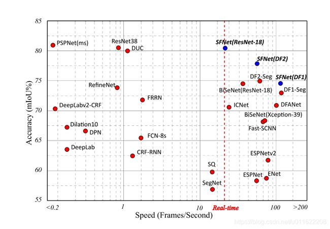
关键词： 当前速度和精度的完美优化，是第一篇在Cityscapes上实现了80.4％的mIoU，帧速率为26 FPS的文章

1. 简介

语义分割，也称为像素级分类问题，其输出和输入分辨率相同（如题图中，左边为2048x1024分辨率的Cityscapes街景图像，输入模型，得到右边同样分辨率的语义图）。由此，语义分割具有两大需求，即高分辨率和高层语义，而这两个需求和卷积网络设计是矛盾的。

卷积网络从输入到输出，会经过多个下采样层（一般为5个，输出原图1/32的特征图），从而逐步扩大视野获取高层语义特征，高层语义特征靠近输出端但分辨率低，高分率特征靠近输入端但语义层次低。高层特征和底层特征都有各自的弱点，各自的分割问题如图１所示，第二行高层特征的分割结果保持了大的语义结构，但小结构丢失严重；第三行低层特征的分割结果保留了丰富的细节，但语义类别预测的很差。

图1

一个自然的想法就是融合高低层特征，取长补短，分割经典工作FCN和U-Net均采用了这个策略，物体检测中常用的特征金字塔网络(FPN)也是采用了该策略。为下文需要，先介绍两类融合策略，一类是FPN，先自下而上获取高层语义特征，再通过自上而下逐步上采样高层语义特征，并融合对应分辨率的下层特征；另一类是HRNet，自下而上包含多个分辨率通路，不同分辨率特征在自下而上过程中及时进行融合。

2. 数据

项目中作者采用了 对训练用的样本50%进行了均匀采样。各个类别的样本统计关系在：cityscapes_train_cv0_tile1024.json中，具体不知道是怎么得出这个json文件的。

logging.info('Class Uniform items per Epoch:%s', str(num_epoch))
num_per_class = int((num_epoch * class_uniform_pct) / num_classes)
num_rand = num_epoch - num_per_class * num_classes
# create random crops
imgs_uniform = random_sampling(imgs, num_rand)

# now add uniform sampling
for class_id in range(num_classes):
    string_format = "cls %d len %d"% (class_id, len(centroids[class_id]))
    logging.info(string_format)
for class_id in range(num_classes):
    centroid_len = len(centroids[class_id])
    if centroid_len == 0:
        pass
    else:
        class_centroids = random_sampling(centroids[class_id], num_per_class)       # 均匀采样
        imgs_uniform.extend(class_centroids)

3. 网络结构

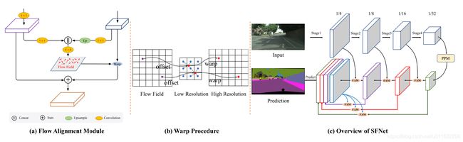
• SFNet去掉FAM模块，再砍掉一些分支之后，其实就和FPN很像，所以其相当于是对FPN的改进（不知道能否用到目标检查上）
• PPM就不具体讲了，可参考:【语义分割】——PSPNET
• PPM多尺度特征之后，就是FAM(光流对齐模块)，这个我们具体讲一下。

code

class AlignedModule(nn.Module):

    def __init__(self, inplane, outplane, kernel_size=3):
        super(AlignedModule, self).__init__()
        self.down_h = nn.Conv2d(inplane, outplane, 1, bias=False)
        self.down_l = nn.Conv2d(inplane, outplane, 1, bias=False)
        self.flow_make = nn.Conv2d(outplane*2, 2, kernel_size=kernel_size, padding=1, bias=False)

    def forward(self, x):
        low_feature, h_feature = x
        h_feature_orign = h_feature
        h, w = low_feature.size()[2:]
        size = (h, w)
        low_feature = self.down_l(low_feature)      # 低层特征 压缩维度
        h_feature= self.down_h(h_feature)           # 高层特征 压缩维度
        h_feature = F.upsample(h_feature, size=size, mode="bilinear", align_corners=True)   # 高层特征上采样
        flow = self.flow_make(torch.cat([h_feature, low_feature], 1))       # 高低层特征融合之后， 光流预测
        h_feature = self.flow_warp(h_feature_orign, flow, size=size)        # 用光流进行上采样

        return h_feature

    def flow_warp(self, input, flow, size):
        out_h, out_w = size
        n, c, h, w = input.size()
        # n, c, h, w
        # n, 2, h, w

        norm = torch.tensor([[[[out_w, out_h]]]]).type_as(input).to(input.device)
        h = torch.linspace(-1.0, 1.0, out_h).view(-1, 1).repeat(1, out_w)
        w = torch.linspace(-1.0, 1.0, out_w).repeat(out_h, 1)               # 50 * 50
        grid = torch.cat((w.unsqueeze(2), h.unsqueeze(2)), 2)               # 50 * 50 * 2
        grid = grid.repeat(n, 1, 1, 1).type_as(input).to(input.device)      # 只用这里的grid的话，就是双线性插值
        grid = grid + flow.permute(0, 2, 3, 1) / norm                       # flow相当于就是特征对齐所需要的采样偏移量

        output = F.grid_sample(input, grid)
        return output

这里的整体流程为：

1. 高层特征，低层特征降维
2. 高层特征上采样，然后，与低层特征融合（到这里和FPN的操作一致）
3. 融合后的特征用于光流预测（这两步是亮点）
4. 用预测的光流进行上采样

预测的光流 shape 为：b × h × w × 2，相当于每个点有两个方向上的偏移量：x，y。然后，预测的光流偏移量flow 再加到 双线性采样的 grid 上（这里flow / norm 相当于归一化的操作）
grid = grid + flow.permute(0, 2, 3, 1) / norm

补充
其实如果只用 grid，那就是双线性插值，但是：待融合的低分辨率高层特征一般通过双线性插值到低层特征的相同分辨率，然后通过相加或沿通道维拼接的方式进行融合。这里引入了两个问题，１．是否每个位置的高低层特征都是同等有效；２．高低层特征空间上存在对不齐的问题，简单上采样无法解决。

其他，模型上就没有什么了。

4. 损失函数

损失函数采用的是：OhemCrossEntropy2dTensor

    def forward(self, pred, target):
        b, c, h, w = pred.size()
        target = target.view(-1)
        valid_mask = target.ne(self.ignore_index)
        target = target * valid_mask.long()
        num_valid = valid_mask.sum()

        prob = F.softmax(pred, dim=1)
        prob = (prob.transpose(0, 1)).reshape(c, -1)
        # ohem 学习，target为前景的点，预测的概率 < threshold 时，才纳入loss计算
        if self.min_kept > num_valid:
            print('Labels: {}'.format(num_valid))
        elif num_valid > 0:
            prob = prob.masked_fill_(~valid_mask, 1)            # 需要被忽略的，填充为1
            mask_prob = prob[
                target, torch.arange(len(target), dtype=torch.long)]        # 根据target选择对应的预测值
            threshold = self.thresh
            if self.min_kept > 0:
                _, index = mask_prob.sort()                     # 升序排列
                threshold_index = index[min(len(index), self.min_kept) - 1]     # 1000个小元素的 threshold
                if mask_prob[threshold_index] > self.thresh:
                    threshold = mask_prob[threshold_index]
                kept_mask = mask_prob.le(threshold)             # 求出小于 threshold 的mask
                target = target * kept_mask.long()
                valid_mask = valid_mask * kept_mask

        target = target.masked_fill_(~valid_mask, self.ignore_index)    # 忽略的 mask 填充为255
        target = target.view(b, h, w)

        return self.criterion(pred, target)

这里是怎么定义ohem的呢？
将 target 为前景的点，该点的预测概率prob < threshold = 0.7 的 index 才用于loss计算。

other

• 用了pytorch的grid_sample操作，不知道能否用tensorrt加速