（sklearn机器学习）第四章_降维算法PCA和SVD

上一章：
下一章：（sklearn机器学习）第五章_逻辑回归（1）https://blog.csdn.net/weixin_45092662/article/details/114537578
PCA算法讲解：https://zhuanlan.zhihu.com/p/77151308
SVD算法讲解：https://zhuanlan.zhihu.com/p/29846048
代码（ipynb）：https://gitee.com/rengarwang/sklearn-machine-learning-code/blob/master/（第四章）降维算法/降维算法.ipynb

对图像的降维可以使用卷积神经网络处理，效果会更好!

调用库和模块

import matplotlib.pyplot as plt
from sklearn.datasets import load_iris
from sklearn.decomposition import PCA

提取数据集

# 提取数据集
iris = load_iris()

# 字典
# iris

y = iris.target
x = iris.data

x.shape

(150, 4)

这是一个2维数组

import pandas as pd 
pd.DataFrame(x)

	0	1	2	3
0	5.1	3.5	1.4	0.2
1	4.9	3.0	1.4	0.2
2	4.7	3.2	1.3	0.2
3	4.6	3.1	1.5	0.2
4	5.0	3.6	1.4	0.2
...	...	...	...	...
145	6.7	3.0	5.2	2.3
146	6.3	2.5	5.0	1.9
147	6.5	3.0	5.2	2.0
148	6.2	3.4	5.4	2.3
149	5.9	3.0	5.1	1.8

150 rows × 4 columns

4维矩阵

建模

# 调用PCA
pca = PCA(n_components=2) #实例化
pca = pca.fit(x) #拟合模型
x_dr = pca.transform(x) #获取新矩阵

# x_dr
# 也可以fit_transform一步到位
# x_dr = PCA(2).fit_transform(x)

x_dr.shape

(150, 2)

可视化

# 要将三种鸢尾花的数据分布显示在二维平面坐标系中，对应的两个坐标（两个特征向量）应该是三种鸢尾花降维后的x1和x2
# 采用布尔索引
x_dr[y == 0, 0]

array([-2.68412563, -2.71414169, -2.88899057, -2.74534286, -2.72871654,
       -2.28085963, -2.82053775, -2.62614497, -2.88638273, -2.6727558 ,
       -2.50694709, -2.61275523, -2.78610927, -3.22380374, -2.64475039,
       -2.38603903, -2.62352788, -2.64829671, -2.19982032, -2.5879864 ,
       -2.31025622, -2.54370523, -3.21593942, -2.30273318, -2.35575405,
       -2.50666891, -2.46882007, -2.56231991, -2.63953472, -2.63198939,
       -2.58739848, -2.4099325 , -2.64886233, -2.59873675, -2.63692688,
       -2.86624165, -2.62523805, -2.80068412, -2.98050204, -2.59000631,
       -2.77010243, -2.84936871, -2.99740655, -2.40561449, -2.20948924,
       -2.71445143, -2.53814826, -2.83946217, -2.54308575, -2.70335978])

colors = ['red','black','orange']
iris.target_names

array(['setosa', 'versicolor', 'virginica'], dtype='

%matplotlib inline
%config InlineBackend.figure_format = 'svg'

plt.figure() # 初始化一个画布
for i in [0, 1, 2]:
    plt.scatter(x_dr[y == i, 0], x_dr[y == i, 1], alpha=0.7, c=colors[i], label=iris.target_names[i])
plt.legend() # 加图例
plt.title('PCA of IRIS dataset') # 加标题
plt.show()

探索降维后的数据

# 查看降维后每个新特征向量上所带的信息量大小（可解释性方差的大小）
pca.explained_variance_

array([4.22824171, 0.24267075])

# 查看降维后每个新特征向量所占的信息量占原始数据总信息量的百分比，又叫做可解释性方差贡献度
pca.explained_variance_ratio_

array([0.92461872, 0.05306648])

pca.explained_variance_ratio_.sum()

0.9776852063187949

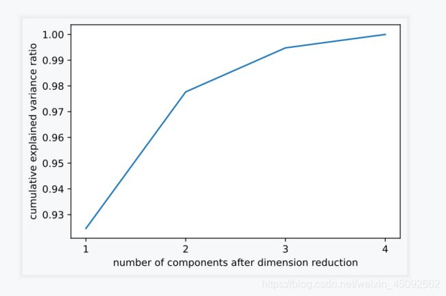
选择最好的n_components

当PCA（）函数中使用默认值时

pca_line = PCA().fit(x)
pca_line.explained_variance_ratio_

array([0.92461872, 0.05306648, 0.01710261, 0.00521218])

import numpy as np 
np.cumsum(pca_line.explained_variance_ratio_)

array([0.92461872, 0.97768521, 0.99478782, 1.        ])

%matplotlib inline
%config InlineBackend.figure_format = 'svg'

plt.plot([1,2,3,4],np.cumsum(pca_line.explained_variance_ratio_))
plt.xticks([1,2,3,4]) # 限制坐标轴显示为整数
plt.xlabel("number of components after dimension reduction")
plt.ylabel("cumulative explained variance ratio")
plt.show()

最大似然估计自选超参数

“mle”自动搜索最佳的n_components，缺点是计算量大。

pca_mle = PCA(n_components="mle")
pca_mle = pca_mle.fit(x)
x_mle = pca_mle.transform(x)

# x_mle

pca_mle.explained_variance_ratio_.sum()

0.9947878161267246

按信息量占比选超参数

假如希望保留97%的信息量,PCA自动选出保留的信息量超过97%的特征数量。

pca_f = PCA(n_components=0.97,svd_solver="full")
pca_f = pca_f.fit(x)
x_f = pca_f.transform(x)

# x_f

pca_f.explained_variance_ratio_

array([0.92461872, 0.05306648])

PCA(2).fit(x).components_

array([[ 0.36138659, -0.08452251,  0.85667061,  0.3582892 ],
       [ 0.65658877,  0.73016143, -0.17337266, -0.07548102]])

PCA(2).fit(x).components_.shape

(2, 4)

PCA中的SVD

降维算法在图像中的应用，PCA中的SVD，卷积神经网络也是一种降维方法

1、导入需要的库和模块

from sklearn.datasets import fetch_lfw_people
from sklearn.decomposition import PCA
import matplotlib.pyplot as plt
import numpy as np

2、实例化数据集

face = fetch_lfw_people(min_faces_per_person=60) # 实例化

# face

7个人的人脸数据集1000多张照片

face.images.shape
# 1348 是矩阵中图像的个数
# 62 是每个图像的特征矩阵的行，像素
# 47 是每个图像的特征矩阵的列，像素

(1348, 62, 47)

face.data.shape
# 行是样本
# 列是样本相关的所有特征

(1348, 2914)

x = face.data

x.shape

(1348, 2914)

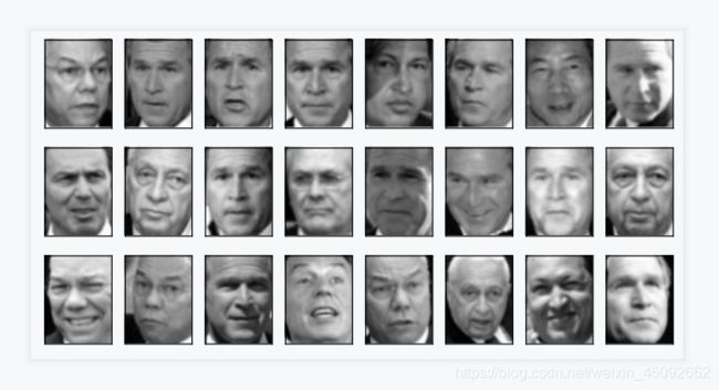
3、将原特征矩阵进行可视化

%matplotlib inline
%config InlineBackend.figure_format = 'svg'

# 创建画布和子图对象
fig, axes = plt.subplots(4,5
                        ,figsize=(8,4) # 图片行和列大小
                        ,subplot_kw={"xticks":[],"yticks":[]} # 不要显示坐标轴
                        )
axes[0][0].imshow(face.images[0,:,:])

axes.shape

(4, 5)

不难发现，axes中的一个对象对应fig中的一个空格

我们希望，在每一个子图对象中填充图像（共20张图），因此我们需要写一个在子图对象中遍历的循环

len([*axes.flat])

20

[*enumerate(axes.flat)]

[(0, ),
 (1, ),
 (2, ),
 (3, ),
 (4, ),
 (5, ),
 (6, ),
 (7, ),
 (8, ),
 (9, ),
 (10, ),
 (11, ),
 (12, ),
 (13, ),
 (14, ),
 (15, ),
 (16, ),
 (17, ),
 (18, ),
 (19, )]

# 填充图像
for i, ax in enumerate(axes.flat):
    ax.imshow(face.images[i,:,:], cmap="gray")

fig, axes = plt.subplots(3,8,figsize=(8,4),subplot_kw = {"xticks":[],"yticks":[]})

for i, ax in enumerate(axes.flat):
    ax.imshow(x[i,:].reshape(62,47),cmap="gray") 

4、建模降维，提取新特征空间矩阵

# 原本有2914维，现在降到150维
pca = PCA(150).fit(x)

x_dr = pca.transform(x) 

x_dr.shape

(1348, 150)

x_dr

array([[ 1143.7627  ,   635.3198  ,   630.6568  , ...,   -59.572582,
          -18.077328,    52.712475],
       [  699.81866 ,  -656.1236  ,   466.91223 , ...,     7.493326,
           49.63772 ,    56.327686],
       [   37.938698,  -270.23184 ,   259.49713 , ...,   -32.80977 ,
           21.706087,   -14.233734],
       ...,
       [ -548.409   ,  -709.99036 ,   127.73023 , ...,    -5.308317,
           58.37268 ,    46.13623 ],
       [-1525.7004  ,  -532.31055 ,   423.82315 , ...,    -9.639832,
          -29.909899,    90.20811 ],
       [  494.39453 ,  -107.04087 ,   357.85406 , ...,   -18.700172,
           19.165699,    17.739117]], dtype=float32)

pca.explained_variance_ratio_

array([0.18776791, 0.14548899, 0.07103531, 0.06026755, 0.05040748,
       0.02936598, 0.02470631, 0.02047521, 0.01968444, 0.01891782,
       0.01560989, 0.01470453, 0.01214074, 0.01095573, 0.01042817,
       0.00972053, 0.00906779, 0.00876521, 0.00813087, 0.00705087,
       0.00682341, 0.00648109, 0.00603545, 0.00578568, 0.00532363,
       0.00520648, 0.00500154, 0.00476372, 0.0045244 , 0.00425308,
       0.00405167, 0.00380145, 0.00360033, 0.00350987, 0.00347687,
       0.00324892, 0.00314407, 0.00310621, 0.00307643, 0.00290165,
       0.00282753, 0.0027487 , 0.00272783, 0.00259985, 0.00246388,
       0.00238214, 0.0023496 , 0.00231576, 0.00227235, 0.00221907,
       0.00210642, 0.00205901, 0.00202986, 0.00200763, 0.00195911,
       0.00195431, 0.00188171, 0.00182909, 0.00176752, 0.00175944,
       0.00174918, 0.00166451, 0.00161346, 0.00158636, 0.00156621,
       0.00152925, 0.00149928, 0.00146113, 0.0014524 , 0.00141118,
       0.00140531, 0.0013644 , 0.0013622 , 0.00131671, 0.00129231,
       0.00125606, 0.00124962, 0.00123174, 0.00120757, 0.0011877 ,
       0.00117422, 0.00115399, 0.00113184, 0.00110208, 0.0010886 ,
       0.00107578, 0.00105294, 0.00103628, 0.00101856, 0.00101126,
       0.00098022, 0.00097883, 0.00095511, 0.00094186, 0.00092627,
       0.00092295, 0.00088963, 0.0008719 , 0.00086035, 0.0008568 ,
       0.00085071, 0.00082558, 0.00081693, 0.00080203, 0.00078521,
       0.00077608, 0.00076442, 0.00074672, 0.00074222, 0.00073652,
       0.00072231, 0.00071129, 0.00070026, 0.00069162, 0.00068861,
       0.00068426, 0.0006741 , 0.00065837, 0.00065216, 0.00063729,
       0.00063108, 0.0006147 , 0.00060969, 0.00060429, 0.00059193,
       0.00058521, 0.00057888, 0.0005681 , 0.00056254, 0.00056106,
       0.00055009, 0.00053875, 0.00053419, 0.00051922, 0.00051649,
       0.0005053 , 0.00050131, 0.00050055, 0.00048855, 0.00047779,
       0.00047487, 0.00047086, 0.00046334, 0.00045583, 0.00045211,
       0.00044193, 0.00043458, 0.00042758, 0.00041827, 0.0004165 ],
      dtype=float32)

pca.explained_variance_ratio_.sum()

0.9456665

v = pca.components_

# v

v.shape

(150, 2914)

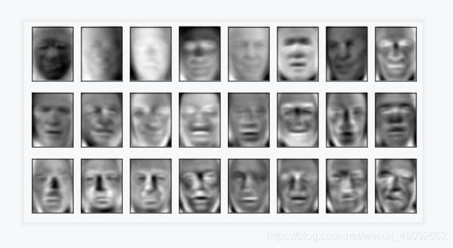
5、将新特征空间矩阵可视化

fig, axes = plt.subplots(3,8,figsize=(8,4),subplot_kw = {"xticks":[],"yticks":[]})

for i, ax in enumerate(axes.flat):
    ax.imshow(v[i,:].reshape(62,47),cmap="gray")

inverse_transform可逆变换

导入模块和库

from sklearn.datasets import fetch_lfw_people
from sklearn.decomposition import PCA
import matplotlib.pyplot as plt
import numpy as np

导入数据

faces = fetch_lfw_people(min_faces_per_person=60)

faces.images.shape

(1348, 62, 47)

faces.data.shape

(1348, 2914)

x = faces.data

建模降维，获取降维后的特征矩阵x_dr

pca = PCA(150)
x_dr = pca.fit_transform(x)

x_dr.shape

(1348, 150)

将降维后矩阵用inverse_transform返回原空间

x_inverse = pca.inverse_transform(x_dr)

x_inverse.shape

(1348, 2914)

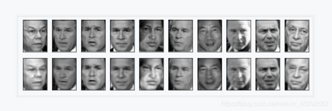
将特征矩阵x和x_inverse可视化

我们需要对子图对象进行遍历的循环，来将图像填入子图中

ax中2行10列，第一行是原始数据，第二行是inverse_transform后返回的数据

需要同时循环两份数据，即一次循环画一列上的两张图，而不是把ax拉平

%matplotlib inline
%config InlineBackend.figure_format = 'svg'

fig, ax = plt.subplots(2,10,figsize=(10,2.5),subplot_kw={"xticks":[],"yticks":[]})
for i in range(10):
    ax[0,i].imshow(faces.images[i,:,:],cmap="binary_r")
    ax[1,i].imshow(x_inverse[i].reshape(62,47),cmap="binary_r")

查看降维后信息量占比

pca.explained_variance_ratio_.sum()

0.94567

可以明显看出，这两组数据可视化后，由降维后再通过inverse_transform转换回原维度的数据画出的图像和原数据画的图大致一样，但愿数据的图像更加清晰。说明数据并没有完全逆转。

这是因为，在降维时，部分信息已经被舍弃了，降维后只有94.56875%的信息被保留，所以在逆转的时候，原数据中已经被舍弃的信息也不可能回来了。所以PCA降维不是完全可逆的。可以设置n_components=300，看看效果。

用PCA做噪声过滤

降维的目的之一就是丢掉对模型带来负面影响的特征。inverse_transform能够在不恢复原始数据的情况下，将降维后的数据返回到原本的高维空间，即“保证维度，但去掉了方差小的特征”。

导入库和模块

from sklearn.datasets import load_digits
from sklearn.decomposition import PCA
import matplotlib.pyplot as plt
import numpy as np

导入数据

digits = load_digits()

digits.data.shape

(1797, 64)

digits.images.shape

(1797, 8, 8)

# digits

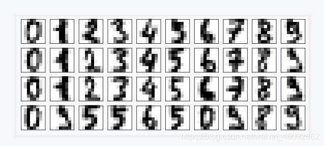
定义画图函数

def plot_digits(data):
    fig, axes = plt.subplots(4,10,figsize=(10,4),subplot_kw={"xticks":[],"yticks":[]})
    for i,ax in enumerate(axes.flat):
        ax.imshow(data[i].reshape(8,8),cmap="binary")
        
plot_digits(digits.data)

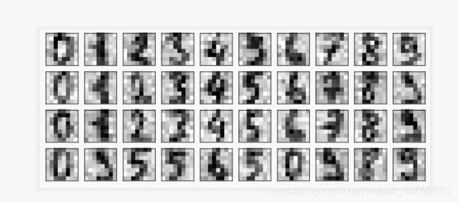
为数据加上噪声

在指定的数据集中，随机抽取服从正态分布的数据

两个参数，分别是指定的数据集，和抽取出来的正态分布的方差

np.random.RandomState(42)
noisy = np.random.normal(digits.data, 2)

plot_digits(noisy)

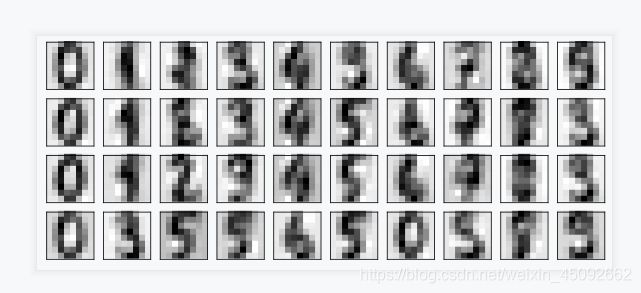
降维

保留信息量为0.5

pca = PCA(0.5).fit(noisy)
x_dr = pca.transform(noisy)
x_dr.shape

(1797, 6)

逆转降维结果，实现降噪

without_noise = pca.inverse_transform(x_dr)
plot_digits(without_noise)

有用请点个赞！！
本站所有文章均为原创，欢迎转载，请注明文章出处：https://blog.csdn.net/weixin_45092662。百度和各类采集站皆不可信，搜索请谨慎鉴别。技术类文章一般都有时效性，本人习惯不定期对自己的博文进行修正和更新，因此请访问出处以查看本文的最新版本。