【书籍阅读 Ch1&2】Reinforcement Learning An Introduction, 2nd Edition
文章目录
- Chapter 1
-
- [Elements] Page:27/548 Date:12/3
- Chapter 2
-
- [Multi-armed Bandits] Page:47&48/548 Date:12/14
- LP28 Figure Code:
- 总结第二章方法 Chapter.2
- All Exercise Part
前言:张聪明的强化学习书籍阅读系列开启 发现博客挖了好多坑没填… 就开新的了(比如上次的文献综述)
这个算是练习笔记了 - 更多是我留下的另一些坑… ?希望大佬们看到了 看懂了能解答一二
每一个目录对应的是在pdf的页数(如果LPage就是书左上角的页码 - 因为我发现后面我要在两页之间加空白页 做练习lol 例如:LPage28 就是左上角书页28页,RPage29就是右上角书页29页);
更新时间:12/24
推荐观看:
1.强化学习 Reinforcement Learning (莫烦 Python 教程)
2.英文 - PDF链接
3 中文 - 官方京东书籍购买链接
代码参考:
1.github 关于整本书的图python代码
Chapter 1
[Elements] Page:27/548 Date:12/3
一个强化学习系统应该具备四个元素:
1. policy (mapping from perceived states of the environment to actions )
也就是environment -> states -> action
policy 可以使随机的 仅指出每个动作的概率【怎么去计算概率呢?】
2. reward signal (确定了强化学习的目标 短期=每一步)
类似于这个动作 (每一个动作后的)reward:a single number 【建一个reward函数】
最大化 the total rewards
3. a value function(长期的 what is good in the long run)
4. model of the environment (optional)
Chapter 2
[Multi-armed Bandits] Page:47&48/548 Date:12/14
首先这里的multi-armed是多个赌博机(单臂->多臂:单臂的多个),所以每一次action对应的就是你动了哪几个赌博机
本章节首先提出的是:RL与其他学习方法不同之处是:仅评价action 不直接给出正确的action
在k-armed中 k个动作对应rewards;也就是动作的评价值(value of action)
在时间t选中的动作为: A t A_t At,对应的rewards就是 R t R_t Rt 对于任意的动作 a a a的评价值都为 q ∗ ( a ) q_*(a) q∗(a)也就是动作a被选中的期待reward
q ∗ ( a ) = E [ R t ∣ A t = a ] q_*(a) = \Bbb{E} [R_t|A_t=a] q∗(a)=E[Rt∣At=a]
LP28 Figure Code:
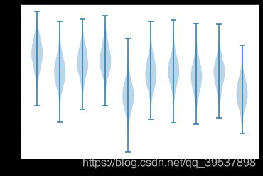
书里写了是10个赌博机(10个action)的2000个随机变量,标准正态分布(mean=0, variance=1 到后面的练习题的时候就不能randn了 因为mean=0, variance =0.01) 图的类型是小提琴图…
import matplotlib
import matplotlib.pyplot as plt
import numpy as np
%matplotlib inline
plt.violinplot(dataset=np.random.randn(2000, 10)+ np.random.randn(10))# uniform distribution + np.random.randn(10))
plt.show()
生成的类似于这种(其中按书的意思是十个bandit就是一个正态分布(10),每一个bandit中再次正态分布所以再加了一次这10个赌博机np.random.randn(2000, 10)呈正态分布,即对于这十个action有好有坏,是个action内,又有2000个正态分布的点

总结第二章方法 Chapter.2
首先是要明确,动作的选择是由最大的Q值来选的,如下公式
A t = ˙ a r g m a x a Q t ( a ) A_t\dot=\mathop {argmax}\limits_a Q_t(a) At=˙aargmaxQt(a)而第二章的内容就是计算Q值的方法有哪几个?到此为止,我们一共有下列几种选择的方法【四种方法均在下面的class Bandit中有代码对应】
然后之所以我画出上一节的Figure 2.1是因为这个至关重要!如果看书LPage28,我们可以大概看出选 q ∗ ( 3 ) q_*(3) q∗(3)是最好的,但是呢, q ∗ ( 3 ) q_*(3) q∗(3)也存在着不好的时候,而我们在选择的时候 实际的收益就是拿阴影段的正态分布,大部分你可以得到1.5(眼看的数据)但是有时候你可能是0.1?最坏的时候-1但是概率很小,概率的分布就是正态的,所以在step()这个函数里,收益的更新reward = np.random.randn() + self.q_true[action]你就知道了+的前后是什么 前是阴影的,后是q3在q1-10里是什么样的整体收益。【希望我解释清楚了这一点 因为当我第一次看这个的时候 疑惑了很久】
- 对应2.2 sample-average
Q t ( a ) = ˙ t 时 刻 前 通 过 执 行 动 作 a 所 得 到 的 收 益 t 时 刻 前 执 行 动 作 a 的 次 数 = ∑ i = 1 t − 1 R i 1 A i = a ∑ i = 1 t − 1 1 A i = a Q_t(a)\dot=\frac{t时刻前通过执行动作a所得到的收益}{t时刻前执行动作a的次数}=\frac{{\sum\limits_{i = 1}^{t - 1} {{R_i}{1_{{A_i} = a}}} }}{{\sum\limits_{i = 1}^{t - 1} {{1_{{A_i} = a}}} }} Qt(a)=˙t时刻前执行动作a的次数t时刻前通过执行动作a所得到的收益=i=1∑t−11Ai=ai=1∑t−1Ri1Ai=a1.1 对应2.4 Incremental Implementation 增量式的实现 [代码对应:constant step size]
Q n = ˙ R 1 + R 2 + ⋯ + R n − 1 n − 1 Q_n\dot=\frac{R_1+R_2+\dotsb+R_{n-1}}{n-1} Qn=˙n−1R1+R2+⋯+Rn−1但是这样计算的就需要存取每一次动作后的收益,内存与计算量会慢慢增加。RPage31中有计算均值过程
Q n + 1 = Q n + 1 n [ R n − Q n ] Q_{n+1}=Q_n+\frac{1}{n}[R_n-Q_n] Qn+1=Qn+n1[Rn−Qn]1.2 对应2.5 收益概率随时间变化 [代码对应:给定step_size并使用包含这个的方法]
在点1.1中我们写出的Q=R的平均,前提是R随时间不发生变化 例如 R 1 R_1 R1如果到了 R n − 1 R_{n-1} Rn−1的时候还会是 R 1 R_1 R1嘛? 在这里我们讨论的就是这个【如果不是 如果会随时间慢慢消退这个第一步收益的影响 而加大后面走向终点的影响是更好的一种方式】在AI课中有时候用discount γ \gamma γ来代表这一意思,所以又可以改写成这样
Q n + 1 = Q n + α [ R n − Q n ] = ( 1 − α ) n Q 1 + ∑ i = 1 n α ( 1 − α ) n − i R i \begin{aligned} Q_{n+1}&=Q_n+ \alpha [R_n-Q_n]\\ &=(1-\alpha)^nQ_1+\sum\limits_{i = 1}^{n}\alpha(1-\alpha)^{n-i}R_i \end{aligned} Qn+1=Qn+α[Rn−Qn]=(1−α)nQ1+i=1∑nα(1−α)n−iRi - 练习2.6中提到的公式( unbiased constant-step-size trick [代码对应: unbiased_constant]
- 对应2.7 Upper-Confidence-Bound Action Selection [代码对应:UCB]
A t = ˙ a r g m a x a [ Q t ( a ) + c ln t N t ( a ) ] {A_t}\dot = \mathop {argmax}\limits_a \left[ {{Q_t}(a) + c\sqrt {\frac{{\ln t}}{{{N_t}(a)}}} } \right] At=˙aargmax[Qt(a)+cNt(a)lnt]利用这个UCB的方法 被选择过的赌博机 对于greedy的状态被选择的机率就会降低,但是这是对optimal方法的改进。 - 对应2.8 gradient
这里是关于bandit的整个代码块:【注释处也有一定的对应关系 可以随着公式一起看】
class Bandit:
    # @k_arm: # of arms
    # @epsilon: probability for exploration in epsilon-greedy algorithm
    # @initial: initial estimation for each action
    # @step_size: constant step size for updating estimations
    # @sample_averages: if True, use sample averages to update estimations instead of constant step size
    # @UCB_param: if not None, use UCB algorithm to select action
    # @gradient: if True, use gradient based bandit algorithm
    # @gradient_baseline: if True, use average reward as baseline for gradient based bandit algorithm
    # @unbiased_constant: things about exercise 2.4 (written by Kin)
    # @ex26: things about exercise 2.6 (written by Kin)
    def __init__(self, k_arm=10, epsilon=0., initial=0., step_size=0.1, sample_averages=False, UCB_param=None,
                 gradient=False, gradient_baseline=False, true_reward=0.,unbiased_constant=False,ex26=False):
        self.k = k_arm
        self.step_size = step_size
        self.sample_averages = sample_averages
        self.unbiased_constant = unbiased_constant
        self.indices = np.arange(self.k)
        self.time = 0
        self.UCB_param = UCB_param
        self.gradient = gradient
        self.gradient_baseline = gradient_baseline
        self.average_reward = 0
        self.true_reward = true_reward
        self.epsilon = epsilon
        self.initial = initial
        self.o_param = 0
        self.ex26 = ex26
    def reset(self):
        # real reward for each action
        if self.ex26:
            self.q_true = np.ones(self.k)*0
        else:
            self.q_true = np.random.randn(self.k) + self.true_reward

        # estimation for each action
        self.q_estimation = np.zeros(self.k) + self.initial

        # # of chosen times for each action
        self.action_count = np.zeros(self.k)

        self.best_action = np.argmax(self.q_true)

        self.time = 0

    # get an action for this bandit
    def act(self):
        if np.random.rand() < self.epsilon:
            return np.random.choice(self.indices)

        if self.UCB_param is not None:
            UCB_estimation = self.q_estimation + \
                self.UCB_param * np.sqrt(np.log(self.time + 1) / (self.action_count + 1e-5))
            q_best = np.max(UCB_estimation)
            return np.random.choice(np.where(UCB_estimation == q_best)[0])

        if self.gradient:
            # 对应公式 (2.11) 更新每个动作被选择的概率
            exp_est = np.exp(self.q_estimation)
            self.action_prob = exp_est / np.sum(exp_est)
            return np.random.choice(self.indices, p=self.action_prob)

        q_best = np.max(self.q_estimation)
        return np.random.choice(np.where(self.q_estimation == q_best)[0])

    # take an action, update estimation for this action
    def step(self, action):
        # generate the reward under N(real reward, 1)
        reward = np.random.randn() + self.q_true[action]
        if self.ex26:
            self.q_true += np.random.normal(0,0.01,self.k)
            self.best_action = np.argmax(self.q_true)
        self.time += 1
        self.action_count[action] += 1
        self.average_reward += (reward - self.average_reward) / self.time

        if self.sample_averages:
            # update estimation using sample averages 对应公式 (2.3) action_count就是n
        	# 这里的action_count是变量 count嘛
            self.q_estimation[action] += (reward - self.q_estimation[action]) / self.action_count[action]

        elif self.unbiased_constant:
            # 这里对应的是练习2.6的公式
            self.q_estimation[action] += self.step_size * (reward - self.q_estimation[action])
            self.o_param += self.step_size * ( 1 - self.o_param )
            self.step_size = self.step_size/self.o_param

        elif self.gradient:
            # 对应公式 (2.11)
            one_hot = np.zeros(self.k)
            one_hot[action] = 1
            if self.gradient_baseline:
                baseline = self.average_reward
            else:
                baseline = 0
            self.q_estimation += self.step_size * (reward - baseline) * (one_hot - self.action_prob)

        else:
            # update estimation with constant step size
            # step_size就是step size说了和没说似乎差不多lol 与2.3的不同之处的
            # 这里的stepsize是常量
            self.q_estimation[action] += self.step_size * (reward - self.q_estimation[action])
        return reward
这里是模拟每一次的step和reward
def simulate(runs, time, bandits):
    rewards = np.zeros((len(bandits), runs, time))
    best_action_counts = np.zeros(rewards.shape)
    for i, bandit in enumerate(bandits):
        for r in trange(runs):
            bandit.reset()
            for t in range(time):
                action = bandit.act()
                reward = bandit.step(action)
                rewards[i, r, t] = reward
                if action == bandit.best_action:
                    best_action_counts[i, r, t] = 1
    mean_best_action_counts = best_action_counts.mean(axis=1)
    mean_rewards = rewards.mean(axis=1)
    return mean_best_action_counts, mean_rewards
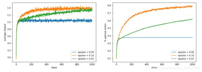
那么进入实操 例如要画出书本Figure 2.2的图, ϵ \epsilon ϵ是0,0.1,0.01进行对比,k=10,1000个time step和2000次独立运行(RPage29)
# 运行区
runs=2000
time=1000
epsilons = [0, 0.1, 0.01]
bandits = [Bandit(epsilon=eps, sample_averages=True) for eps in epsilons]
best_action_counts, rewards = simulate(runs, time, bandits)

# 画图区
plt.figure(figsize=(10, 20))
plt.subplot(2, 1, 1)
for eps, rewards in zip(epsilons, rewards):
    plt.plot(rewards, label='epsilon = %.02f' % (eps))
plt.xlabel('steps')
plt.ylabel('average reward')
plt.legend()

plt.subplot(2, 1, 2)
for eps, counts in zip(epsilons, best_action_counts):
    plt.plot(counts, label='epsilon = %.02f' % (eps))
plt.xlabel('steps')
plt.ylabel('% optimal action')
plt.legend()
All Exercise Part
Exercise 2.1:In ε ε ε-greedy action selection, for the case of two actions and ε ε ε = 0.5, what is the probability that the greedy action is selected?
50%
理由:ε的选择就是 prob>ε 选择exploration;prob<ε的时候选择当前最好的,五五开所以 被选择的概率也五五开
Exercise 2.2: Bandit example Consider a k-armed bandit problem with k = 4 actions, denoted 1, 2, 3, and 4. Consider applying to this problem a bandit algorithm using ε-greedy action selection, sample-average action-value estimates, and initial estimates of Q 1 ( a ) = 0 Q_1(a) = 0 Q1(a)=0, for all a. Suppose the initial sequence of actions and rewards is A 1 = 1 , R 1 = − 1 , A 2 = 2 , R 2 = 1 , A 3 = 2 , R 3 = − 2 , A 4 = 2 , R 4 = 2 , A 5 = 3 , R 5 = 0 A_1 = 1, R_1 = -1, A_2 = 2, R_2 = 1, A_3 = 2, R_3 = -2, A_4 = 2, R_4 = 2, A_5 = 3, R_5 = 0 A1=1,R1=−1,A2=2,R2=1,A3=2,R3=−2,A4=2,R4=2,A5=3,R5=0. On some of these time steps the ε \varepsilon ε case may have occurred, causing an action to be selected at random. On which time steps did this definitely occur? On which time steps could this possibly have occurred?
Definite: t2, t5; Possible: t1, t3
Reason:
2.1.1
Here in time step 2, the exploratory action occurred since it has observed that action 1 yielded reward 1 which is greater than 0 for the other actions. It definitely occurred at time step 5 since the reward is 0 and it wasn’t the greedy choice of action 2.
2.1.2
At timestep 2 2 2 this definitely occurred, as we know that the average reward associated with A 1 A_1 A1 is 1 1 1 and so Q 2 ( a 1 ) > Q 2 ( a 2 ) = 0 Q_2(a_1) >Q_2(a_2) = 0 Q2(a1)>Q2(a2)=0. Therefore, choosing A 2 = 2 A_2 = 2 A2=2 must have been the result of a exploration step. Similarly, this must have also occurred at timestep 5 5 5.
It might have occurred at timestep 1 1 1, depending on how the algorithm picks among actions with equal Q Q Q values. The same is true for timestep 3 3 3, at the beginning of which a 2 a_2 a2 and a 1 a_1 a1 have the same Q Q Q value.
If when one is picking a random action, one chooses among all actions rather than just all the ones currently considered suboptimal, then it is possible that a random action was selected at any of the timesteps.
【问题:如果是这样的话,那action有关吗?t=5的时候因为比t=4最大的小,所以一定探索?那为啥t=4直接选了?不存在探索的可能性?】
2.1.3我的解释:How to understand k-armed bandit example from Sutton’s RL book chapter 2?
Here is the table:
| Time | Action ( A i A_i Ai) | Reward ( R i R_i Ri) |
|---|---|---|
| 1 | 1 | -1 |
| 2 | 2 | 1 |
| 3 | 2 | -2 |
| 4 | 2 | 2 |
| 5 | 3 | 0 |
My explanation:
First, convert Reward to Q:
Q t ( a ) = ∑ i = 1 t − 1 R i 1 A i = a ∑ i = 1 t − 1 1 A i = a {Q_t}(a) = \frac{{\sum\limits_{i = 1}^{t - 1} {{R_i}{1_{{A_i} = a}}} }}{{\sum\limits_{i = 1}^{t - 1} {{1_{{A_i} = a}}} }} Qt(a)=i=1∑t−11Ai=ai=1∑t−1Ri1Ai=a
| Iteration = Time | Q(1) | Q(2) | Q(3) | Q(4) |
|---|---|---|---|---|
| 0 | 0 | 0 | 0 | 0 |
| 1 | -1 | 0 | 0 | 0 |
| 2 | -1 | 1 | 0 | 0 |
| 3 | -1 | -0.5 | 0 | 0 |
| 4 | -1 | 1/3 | 0 | 0 |
| 5 | -1 | 1/3 | 0 | 0 |
So at time1 & time3 there are more than one max action (possible occur)
time2,4,5 we have the max Q value which response to action 2
But I still have problems with time 4 since I found other blog which said time 4 does not definitely occur, and also about the ε \varepsilon ε case it’s about the probability what’s the meaning about the question must occur?
主要是我发现好像… 大家复制问问题的时候都丢掉了负号,所以答案不一定了…
Exercise 2.3: In the comparison shown in Figure 2.2, which method will perform best in the long run in terms of cumulative reward and probability of selecting the best action? How much better will it be? Express your answer quantitatively.
e of 0.01% will perform better in the long run as it will end up choosing the correct actions 99.1% of the time,versus 91% of the time for e of 0.1%, a difference of 8.1%
【问题:91%在书左上角P30页,99.1%是怎么得出来的?】
Ref:
2.1.1Multi-Armed Bandits
2.1.2Sutton & Barto - Reinforcement Learning: Some Notes and Exercises
2.2 rlai-exercises
Exercise 2.4: If the step-size parameters, α n α_n αn, are not constant, then the estimate Q n Q_n Qn is a weighted average of previously received rewards with a weighting different from that given by (2.6). What is the weighting on each prior reward for the general case, analogous to (2.6), in terms of the sequence of step-size parameters?
解答如图:

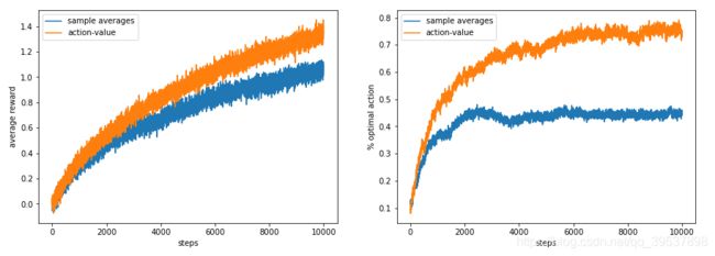
Exercise 2.5 (programming): Design and conduct an experiment to demonstrate the difficulties that sample-average methods have for nonstationary problems. Use a modified version of the 10-armed testbed in which all the q(a) start out equal and then take independent random walks (say by adding a normally distributed increment with mean zero and standard deviation 0.01 to all the q(a) on each step). Prepare plots like Figure 2.2 for an action-value method using sample averages, incrementally computed, and another action-value method using a constant step-size parameter, α = 0.1. Use ε = 0.1 and longer runs, say of 10,000 steps.
到这里我假设大家都熟悉了上面提到的class bandit这个类了哈,那我就开始写这个练习的情况下的代码了:对于代码的修改:
首先是step()里的 best_action会变,因为题目中说了 all the q(a) start out equal and then take independent random walks (add mean=0 variance=0.01)的,对应这句话进行q_true的更新
# code in def step():
        if self.ex26:
            self.q_true += np.random.normal(0,0.01,self.k)
            self.best_action = np.argmax(self.q_true)
#parameters
runs=2000
time=1000

#Run bandits
bandits = [Bandit(epsilon=0.1, sample_averages=True,true_reward=np.random.normal(0,0.01)),
           Bandit(epsilon=0.1, step_size=0.1,sample_averages=False,true_reward=np.random.normal(0,0.01))]
best_action_counts, rewards = simulate(runs, time, bandits)

# Plot
plt.figure(figsize=(10, 20))
plt.subplot(2, 1, 1)
for labelp,rp in zip(['sample averages','action-value'],rewards):
    plt.plot(rp,label=labelp)
plt.xlabel('steps')
plt.ylabel('average reward')
plt.legend()

plt.subplot(2, 1, 2)
for labelp,counts in zip(['sample averages','action-value'],best_action_counts):
    plt.plot(counts,label=labelp)
plt.xlabel('steps')
plt.ylabel('% optimal action')
plt.legend()
Exercise 2.6: Mysterious Spikes The results shown in Figure 2.3 should be quite reliable because they are averages over 2000 individual, randomly chosen 10-armed bandit tasks. Why, then, are there oscillations and spikes in the early part of the curve for the optimistic method? In other words, what might make this method perform particularly better or worse, on average, on particular early steps?
When the initial action value is set to be larger than its mean, agent might pull a good arm by chance and then update the estimates, the estimate will decrease with large probability. since it’s the begining phase, some worse arms might haven’t been played thus their action value haven’t been updated, therefore larger than the updated good arms. Under the greedy frame, the agent will play these ”worse” arms and update. Hence results in the spikes in the figure.
Possible way to improve: If at the initialization, assign larger action values to better arms and smaller value to worse arm.
Possible way to worsen the case: Action values assigned to worse arms are larger than arms with higher expected reward.
Exercise 2.7: Unbiased Constant-Step-Size Trick In most of this chapter we have used sample averages to estimate action values because sample averages do not produce the initial bias that constant step sizes do (see the analysis leading to (2.6)). However, sample averages are not a completely satisfactory solution because they may perform poorly on nonstationary problems. Is it possible to avoid the bias of constant step sizes while retaining their advantages on nonstationary problems? One way is to use a step size of
β n . = α / o ¯ n βn .= α/o¯n βn.=α/o¯nto process the nth reward for a particular action, where α > 0 α > 0 α>0 is a conventional constant step size, and o ^ n \hat o_n o^n is a trace of one that starts at 0:
o ¯ n . = ¯ o n 1 + α ( 1 o ¯ n 1 ) , f o r n 0 , w i t h ¯ o 0. = 0 o¯n .= ¯on1 + α(1 o¯n1), for n 0, with ¯o0 .= 0 o¯n.=¯on1+α(1o¯n1),forn0,with¯o0.=0Carry out an analysis like that in (2.6) to show that Q n Q_n Qn is an exponential recency-weighted average without initial bias.
Exercise 2.8: UCB Spikes In Figure 2.4 the UCB algorithm shows a distinct spike in performance on the 11th step. Why is this? Note that for your answer to be fully satisfactory it must explain both why the reward increases on the 11th step and why it decreases on the subsequent steps. Hint: if c = 1, then the spike is less prominent.
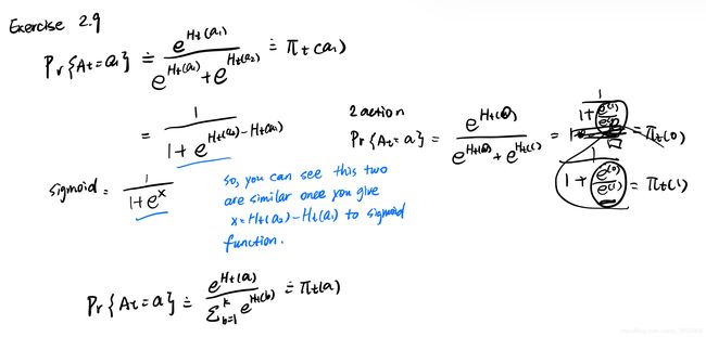
Exercise 2.9: Show that in the case of two actions, the soft-max distribution is the same as that given by the logistic, or sigmoid, function often used in statistics and artificial neural networks.
解答如图:

Exercise 2.10: Suppose you face a 2-armed bandit task whose true action values change randomly from time step to time step. Specifically, suppose that, for any time step, the true values of actions 1 and 2 are respectively 0.1 and 0.2 with probability 0.5 (case A), and 0.9 and 0.8 with probability 0.5 (case B). If you are not able to tell which case you face at any step, what is the best expectation of success you can achieve and how should you behave to achieve it? Now suppose that on each step you are told whether you are facing case A or case B (although you still don’t know the true action values). This is an associative search task. What is the best expectation of success you can achieve in this task, and how should you behave to achieve it?
For the first scenario, you cannot hold individual estimates for the case A and B. Therefore, the best approach is to select the action that has best value estimate in combination. In this case, the estimates of both actions the same. So the best expectation of success is 0.5 and it can be achieved by selecting an action randomly at each step.
A 1 = 0.5 ∗ 0.1 + 0.5 ∗ 0.9 = 0.5 A1 = 0.5 * 0.1 + 0.5 * 0.9 = 0.5 A1=0.5∗0.1+0.5∗0.9=0.5
A 2 = 0.5 ∗ 0.2 + 0.5 ∗ 0.8 = 0.5 A2 = 0.5 * 0.2 + 0.5 * 0.8 = 0.5 A2=0.5∗0.2+0.5∗0.8=0.5
For the second scenario, you can hold independent estimates for the case A and B, thus we can learn the best action for each one treating them as independent bandit problems. The best expectation of success is 0.55 obtained from selecting A2 in case A and A1 in case B.
0.5 ∗ 0.2 + 0.5 ∗ 0.9 = 0.55 0.5 * 0.2 + 0.5 * 0.9 = 0.55 0.5∗0.2+0.5∗0.9=0.55
Ref:
1.github 关于整本书的图python代码
2.github上的部分Reinforcement-Learning-2nd-Edition-by-Sutton-Exercise-Solutions

