莫烦pytorch学习笔记4
莫烦pytorch学习笔记4
- 1 卷积网络
- 2 循环神经网络RNN,LSTM,GRU
-
- 2.1 RNN
- 2.2 LSTM
- 2.3 RNN分类例子
- 2.4 RNN回归例子
- 2.5 logistic 回归
1 卷积网络
理论:https://blog.csdn.net/weixin_41781408/article/details/88578849
import torch
import torch.nn as nn
from torch.autograd import Variable
import torch.utils.data as Data
import torchvision
import matplotlib.pyplot as plt


# Hyper Parameters
EPOCH = 1               # train the training data n times, to save time, we just train 1 epoch
BATCH_SIZE = 50
LR = 0.001              # learning rate
DOWNLOAD_MNIST = True   # set to False if you have downloaded
# Mnist digits dataset
train_data = torchvision.datasets.MNIST(
    root='./mnist/',
    train=True,                                     # this is training data
    transform=torchvision.transforms.ToTensor(),    # Converts a PIL.Image or numpy.ndarray to
                                                    # torch.FloatTensor of shape (C x H x W) and normalize in the range [0.0, 1.0]
    download=DOWNLOAD_MNIST,                        # download it if you don't have it
)
# plot one example
print(train_data.train_data.size())                 # (60000, 28, 28)
print(train_data.train_labels.size())               # (60000)
# plt.imshow(train_data.train_data[0].numpy(), cmap='gray')
# plt.title('%i' % train_data.train_labels[0])
# plt.show()

train_loader = Data.DataLoader(
    dataset=train_data,
    batch_size=BATCH_SIZE,
    shuffle=True)

# convert test data into Variable, pick 2000 samples to speed up testing
test_data = torchvision.datasets.MNIST(root='./mnist/', train=False)
test_x = Variable(torch.unsqueeze(test_data.test_data, dim=1)).type(torch.FloatTensor)[:2000]/255.   # shape from (2000, 28, 28) to (2000, 1, 28, 28), value in range(0,1)
test_y = test_data.test_labels[:2000]
class CNN(nn.Module):
    def __init__(self):
        super(CNN, self).__init__()
        self.conv1 = nn.Sequential(         # input shape (1, 28, 28)
            nn.Conv2d(
                in_channels=1,              # input height 有几层 rgb 三层 灰度图1层
                out_channels=16,            # n_filters  输出层 16 层 想象 1层变成16层
                kernel_size=5,              # filter size 这个卷积核的大小5X5
                stride=1,                   # filter movement/step  #移动步子 大小
                padding=2,                  # if want same width and length of this image after con2d, padding=(kernel_size-1)/2 if stride=1 使的输出的层大小和卷积之前一样
            ),                              # output shape (16, 28, 28)
            nn.ReLU(),                      # activation
            nn.MaxPool2d(kernel_size=2),    # choose max value in 2x2 area, output shape (16, 14, 14)
        )
        self.conv2 = nn.Sequential(         # input shape (1, 28, 28)
            nn.Conv2d(16, 32, 5, 1, 2),     # ou tput shape (32, 14, 14) 输入16 层 14X14 输出 32层 14X14
            nn.ReLU(),                      # activation
            nn.MaxPool2d(2),                # output shape (32, 7, 7) 32层 14X14
        )
        self.out = nn.Linear(32 * 7 * 7, 10)   # fully connected layer, output 10 classes 全连接 32X14X14 输出10

    def forward(self, x):
        x = self.conv1(x)
        x = self.conv2(x)  #(batch,32,7,7)
        x = x.view(x.size(0), -1)           # flatten the output of conv2 to (batch_size, 32 * 7 * 7)
        output = self.out(x)
        return output, x    # return x for visualization
cnn=CNN()
optimizer = torch.optim.SGD(cnn.parameters(), lr=LR)
loss_func = torch.nn.CrossEntropyLoss()  # the target label is NOT an one-hotted

for epoch in range(EPOCH):   # train entire dataset 3 times
    for step, (x, y) in enumerate(train_loader):  # for each training step
        # train your data...
        b_x = Variable(x)  # batch x
        b_y = Variable(y)  # batch y
        output = cnn(b_x)[0]  # cnn output
        loss = loss_func(output, b_y)  # cross entropy loss
        optimizer.zero_grad()  # clear gradients for this training step
        loss.backward()  # backpropagation, compute gradients
        optimizer.step()
        if step % 100 == 0:
            test_output, last_layer = cnn(test_x)
            pred_y = torch.max(test_output, 1)[1].data.squeeze()
            accuracy = (pred_y == test_y).sum().item() / float(test_y.size(0))
            print('Epoch: ',epoch, '|step',step,'| train loss: %.4f' % loss.data, '| test accuracy: %.2f' % accuracy)


torch.save(cnn,'cnn.pkl')
cnn2=torch.load('cnn.pkl')
test_output,_=cnn(test_x[:10])
pred_y = torch.max(test_output, 1)[1].data.squeeze()
print(pred_y,'预测')
print(test_y[:10])
# prdict,_=cnn2(ptest_x)
# print(prdict)
# plt.imshow(prdict.numpy(), cmap='gray')
# print(type(prdict))
# plt.imshow(test_data.test_data[0].numpy(), cmap='gray')
# plt.show()
2 循环神经网络RNN,LSTM,GRU
理论 :https://blog.csdn.net/weixin_41781408/article/details/88617533
2.1 RNN
如果w 小于1 可能因为步数多而梯度消失,w大于1 可能梯度爆炸。
2.2 LSTM

2.3 RNN分类例子
import torch
from torch import nn
from torch.autograd import Variable
import torchvision.datasets as dsets
import torchvision.transforms as transforms
import matplotlib.pyplot as plt
torch.manual_seed(1) # reproducible
# Hyper Parameters
EPOCH = 1 # train the training data n times, to save time, we just train 1 epoch
BATCH_SIZE = 64
TIME_STEP = 28 # rnn time step / image height
INPUT_SIZE = 28 # rnn input size / image width
LR = 0.01 # learning rate
DOWNLOAD_MNIST = False # set to True if haven't download the data
# Mnist digital dataset
train_data = dsets.MNIST(
root='./mnist/',
train=True, # this is training data
transform=transforms.ToTensor(), # Converts a PIL.Image or numpy.ndarray to
# torch.FloatTensor of shape (C x H x W) and normalize in the range [0.0, 1.0]
download=DOWNLOAD_MNIST, # download it if you don't have it
)
# Data Loader for easy mini-batch return in training
train_loader = torch.utils.data.DataLoader(dataset=train_data, batch_size=BATCH_SIZE, shuffle=True)
# convert test data into Variable, pick 2000 samples to speed up testing
test_data = dsets.MNIST(root='./mnist/', train=False, transform=transforms.ToTensor())
test_x = Variable(test_data.test_data, volatile=True).type(torch.FloatTensor)[:2000]/255. # shape (2000, 28, 28) value in range(0,1)
test_y = test_data.test_labels.numpy().squeeze()[:2000] # covert to numpy array
class RNN(nn.Module):
def __init__(self):
super(RNN, self).__init__()
self.rnn = nn.LSTM( # if use nn.RNN(), it hardly learns
input_size=INPUT_SIZE, #每个时间点28
hidden_size=64, # rnn hidden unit
num_layers=1, # number of rnn layer
batch_first=True, # input & output will has batch size as 1s dimension. e.g. (batch, time_step, input_size)
)
# (time_step,batch,input) batch_first=False
self.out = nn.Linear(64, 10)
def forward(self, x):
# x shape (batch, time_step, input_size)
# r_out shape (batch, time_step, output_size)
# h_n shape (n_layers, batch, hidden_size)
# h_c shape (n_layers, batch, hidden_size)
r_out, (h_n, h_c) = self.rnn(x, None) # None represents zero initial hidden state NOne hiddle_state 状态没有
# (batch,time_step,input_size)
# choose r_out at the last time step
out = self.out(r_out[:, -1, :]) #最后时刻一个状态(batch,time_step,input)
return out
rnn=RNN()
print(rnn)
optimizer=torch.optim.Adam(rnn.parameters(),lr=LR)
loss_func=nn.CrossEntropyLoss()
for i in range(EPOCH):
for step, (x, y) in enumerate(train_loader): # for each training step
b_x = Variable(x.view(-1, 28, 28)) # batch x
b_y = Variable(y) # batch y
output = rnn(b_x) # cnn output
loss = loss_func(output, b_y) # cross entropy loss
optimizer.zero_grad() # clear gradients for this training step
loss.backward() # backpropagation, compute gradients
optimizer.step()
if step % 50 == 0:
test_output = rnn(test_x) # (samples, time_step, input_size)
pred_y = torch.max(test_output, 1)[1].data.numpy().squeeze()
accuracy = sum(pred_y == test_y) / float(test_y.size)
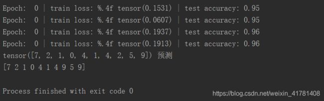
print('Epoch: ', EPOCH,'| train loss:',loss.data, '| test accuracy:' ,accuracy)
torch.save(rnn,'rnnc.pkl')
rnn2=torch.load('rnnc.pkl')
test_output,_=rnn(test_x[:10])
pred_y = torch.max(test_output, 1)[1].data.squeeze()
print(pred_y,'预测')
print(test_y[:10])
2.4 RNN回归例子
import torch
from torch import nn
from torch.autograd import Variable
import numpy as np
import matplotlib.pyplot as plt
torch.manual_seed(1)    # reproducible

# Hyper Parameters
TIME_STEP = 10      # rnn time step
INPUT_SIZE = 1      # rnn input size
LR = 0.02           # learning rate


# show data
steps = np.linspace(0, np.pi*2, 100, dtype=np.float32)
x_np = np.sin(steps)    # float32 for converting torch FloatTensor
y_np = np.cos(steps)
plt.plot(steps, y_np, 'r-', label='target (cos)')
plt.plot(steps, x_np, 'b-', label='input (sin)')
plt.legend(loc='best')
plt.show()

class RNN(nn.Module):
    def __init__(self):
        super(RNN, self).__init__()

        self.rnn = nn.RNN(
            input_size=INPUT_SIZE,
            hidden_size=32,     # rnn hidden unit
            num_layers=1,       # number of rnn layer
            batch_first=True,   # input & output will has batch size as 1s dimension. e.g. (batch, time_step, input_size)
        )
        self.out = nn.Linear(32, 1)

    def forward(self, x, h_state):
        # x (batch, time_step, input_size)
        # h_state (n_layers, batch, hidden_size)
        # r_out (batch, time_step, hidden_size)
        r_out, h_state = self.rnn(x, h_state)

        outs = []    # save all predictions
        for time_step in range(r_out.size(1)):    # calculate output for each time step
            outs.append(self.out(r_out[:, time_step, :]))
        return torch.stack(outs, dim=1), h_state
rnn = RNN()
print(rnn)
optimizer = torch.optim.Adam(rnn.parameters(), lr=LR)   # optimize all cnn parameters
loss_func = nn.MSELoss()

h_state = None      # for initial hidden state

plt.figure(1, figsize=(12, 5))
plt.ion()           # continuously plot

for step in range(60):
    start, end = step * np.pi, (step+1)*np.pi   # time range
    # use sin predicts cos
    steps = np.linspace(start, end, TIME_STEP, dtype=np.float32)
    x_np = np.sin(steps)    # float32 for converting torch FloatTensor
    y_np = np.cos(steps)

    x = Variable(torch.from_numpy(x_np[np.newaxis, :, np.newaxis]))    # shape (batch, time_step, input_size)
    y = Variable(torch.from_numpy(y_np[np.newaxis, :, np.newaxis]))

    prediction, h_state = rnn(x, h_state)   # rnn output
    # !! next step is important !!
    h_state = Variable(h_state.data)        # repack the hidden state, break the connection from last iteration

    loss = loss_func(prediction, y)         # cross entropy loss
    optimizer.zero_grad()                   # clear gradients for this training step
    loss.backward()                         # backpropagation, compute gradients
    optimizer.step()                        # apply gradients

    # plotting
    plt.plot(steps, y_np.flatten(), 'r-')
    plt.plot(steps, prediction.data.numpy().flatten(), 'b-')
    plt.draw(); plt.pause(0.05)

2.5 logistic 回归
import torch
from torch.autograd import Variable
import torch.nn as nn

n_data = torch.ones(100, 2)         # 数据的基本形态
x0 = torch.normal(2*n_data, 1)      # 类型0 x data (tensor), shape=(100, 2)
y0 = torch.zeros(100)               # 类型0 y data (tensor), shape=(100, 1)
x1 = torch.normal(-2*n_data, 1)     # 类型1 x data (tensor), shape=(100, 1)
y1 = torch.ones(100)                # 类型1 y data (tensor), shape=(100, 1)

# 注意 x, y 数据的数据形式是一定要像下面一样 (torch.cat 是在合并数据)
x = torch.cat((x0, x1), 0).type(torch.FloatTensor)  # FloatTensor = 32-bit floating
y = torch.cat((y0, y1), 0).type(torch.FloatTensor)
class LogisticRegression(nn.Module):
    def __init__(self):
        super(LogisticRegression, self).__init__()
        self.lr = nn.Linear(2, 1)
        self.sm = nn.Sigmoid()

    def forward(self, x):
        x = self.lr(x)
        x = self.sm(x)
        return x

logistic_model = LogisticRegression()
if torch.cuda.is_available():
    logistic_model.cuda()

# 定义损失函数和优化器
criterion = nn.BCELoss()
optimizer = torch.optim.SGD(logistic_model.parameters(), lr=1e-3, momentum=0.9)
# 开始训练
for epoch in range(10000):
    if torch.cuda.is_available():
        x_data = Variable(x).cuda()
        y_data = Variable(y).cuda()
    else:
        x_data = Variable(x)
        y_data = Variable(y)

    out = logistic_model(x_data)
    loss = criterion(out, y_data)
    print_loss = loss.data.item()
    mask = out.ge(0.5).float()  # 以0.5为阈值进行分类
    correct = (mask == y_data).sum()  # 计算正确预测的样本个数
    acc = correct.item() / x_data.size(0)  # 计算精度
    optimizer.zero_grad()
    loss.backward()
    optimizer.step()
    # 每隔20轮打印一下当前的误差和精度
    if (epoch + 1) % 20 == 0:
        print('*'*10)
        print('epoch {}'.format(epoch+1)) # 训练轮数
        print('loss is {:.4f}'.format(print_loss))  # 误差
        print('acc is {:.4f}'.format(acc))  # 精度