【4-网络八股扩展】北京大学TensorFlow2.0

课程地址：【北京大学】Tensorflow2.0_哔哩哔哩_bilibili

Python3.7和TensorFlow2.1

六讲：

1. 神经网络计算：神经网络的计算过程，搭建第一个神经网络模型

2. 神经网络优化：神经网络的优化方法，掌握学习率、激活函数、损失函数和正则化的使用，用Python语言写出SGD、Momentum、Adagrad、RMSProp、Adam五种反向传播优化器

3. 神经网络八股：神经网络搭建八股，六步法写出手写数字识别训练模型

4. 网络八股扩展：神经网络八股扩展，增加自制数据集、数据增强、断点续训、参数提取和acc/loss可视化，实现给图识物的应用程序

5. 卷积神经网络：用基础CNN、LeNet、AlexNet、VGGNet、InceptionNet和ResNet实现图像识别

6. 循环神经网络：用基础RNN、LSTM、GRU实现股票预测

---

上一讲：六步法搭建神经网络八股（tf.keras），使用MNIST数据集和FASHION数据集训练网络参数，提升识别准确率

1. import

2. train，test：需要引入训练集输入特征及标签，测试集输入特征及标签，都是用别人打包好的数据集，直接调用 .load_data() 函数实现加载

mnist = tf.keras.datasets.mnist
(x_train, y_train), (x_test, y_test) = mnist.load_data()

• 当使用自制数据集解决本领域应用时，怎么给x_train, y_train, x_test, y_test赋值

• 若数据量过小，模型泛化力弱，如何做数据增强，扩展数据，提高泛化力

3. Sequential / class

model = tf.keras.models.Sequential()
或
class MyModel(Model):
    ...
model = Mymodel()   # 定义模型

4. model.compile 配置模型

5. model.fit 训练模型

• 若每次模型训练都从0开始，十分不划算 —— 断点续训，实时保存最优模型

6. model.summary

• 神经网络训练的目的就是获取各层网络最优的参数，只要拿到这些参数，可以在各个平台实现前向推理，复现出模型，实现应用的 —— 参数提取，把参数存入文本

• acc和loss曲线可以见证模型的优化过程 —— acc/loss可视化，查看训练效果

前向推理实现应用：给图识物的应用程序，输入神经网络一组新的、从未见过的特征，输出预测结果

本讲：

1. 自制数据集，解决本领域应用

2. 数据增强，扩充数据集

3. 断点续训，存取模型

4. 参数提取，把参数存入文本

5. acc/loss可视化，查看训练效果

6. 应用程序，实现给图识物

本讲所有代码baseline均为MNIST分类（Sequential版）的代码，5个epoch后最终测试集的损失为0.0813，准确率为97.53%。完整代码见：【3-神经网络八股】北京大学TensorFlow2.0 - CSDN

---

自制数据集，解决本领域应用

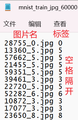
mnist_image_label文件夹：

下面代码只贴出相比baseline改动的部分：

# PIL是Python中常用的图像处理库，提供了诸如图像打开、缩放、旋转、颜色转换等常用功能
from PIL import Image   # 从PIL(Python Imaging Library)模块中导入Image类
import numpy as np
import os

train_path = './mnist_image_label/mnist_train_jpg_60000/'     # 训练集图片路径
train_txt = './mnist_image_label/mnist_train_jpg_60000.txt'   # 训练集标签文件
# 在使用训练好的模型时，有一种保存模型的文件格式叫.npy，是numpy专用的二进制文件
x_train_savepath = './mnist_image_label/mnist_x_train.npy'    # 训练集输入特征存储文件
y_train_savepath = './mnist_image_label/mnist_y_train.npy'    # 训练集标签存储文件

test_path = './mnist_image_label/mnist_test_jpg_10000/'     # 测试集图片路径
test_txt = './mnist_image_label/mnist_test_jpg_10000.txt'   # 测试集标签文件
x_test_savepath = './mnist_image_label/mnist_x_test.npy'    # 测试集输入特征存储文件
y_test_savepath = './mnist_image_label/mnist_y_test.npy'    # 测试集标签存储文件

def generateds(path, txt):    # path为图片路径，txt为标签文件
    f = open(txt, 'r')  # 以只读形式打开txt文件
    contents = f.readlines()  # 读取文件中所有行
    f.close()  # 关闭txt文件
    x, y_ = [], []  # 建立空列表
    for content in contents:  # 逐行取出
        value = content.split()  # 以空格分开，图片路径为value[0] , 标签为value[1] , 存入列表
        img_path = path + value[0]  # 拼出图片路径和文件名，为图片的索引路径
        img = Image.open(img_path)  # 读入图片
        # image = image.convert()是图像实例对象的一个方法，接受一个mode参数，用以指定一种色彩模式
        img = np.array(img.convert('L'))  # 图片变为8位宽度的灰度值，np.array格式
        img = img / 255.  # 数据归一化 （实现预处理）
        x.append(img)  # 归一化后的数据，贴到列表x
        y_.append(value[1])  # 标签贴到列表y_
        print('loading : ' + content)  # 打印状态提示
    x = np.array(x)  # 变为np.array格式
    y_ = np.array(y_)  # 变为np.array格式
    # arr.astype(“具体的数据类型”) 转换numpy数组的数据类型
    y_ = y_.astype(np.int64)  # 变为64位整型
    return x, y_  # 返回输入特征x，标签y_

# 判断训练集输入特征x_train和标签y_train、测试集输入特征x_test和标签y_test是否已存在
if os.path.exists(x_train_savepath) and os.path.exists(y_train_savepath) and os.path.exists(
        x_test_savepath) and os.path.exists(y_test_savepath):
    print('-------------Load Datasets-----------------')    # 若存在，直接读取
    x_train_save = np.load(x_train_savepath)
    y_train = np.load(y_train_savepath)
    x_test_save = np.load(x_test_savepath)
    y_test = np.load(y_test_savepath)
    x_train = np.reshape(x_train_save, (len(x_train_save), 28, 28))
    x_test = np.reshape(x_test_save, (len(x_test_save), 28, 28))
else:   # 若不存在，调用generateds(path, txt)函数制作数据集
    print('-------------Generate Datasets-----------------')
    x_train, y_train = generateds(train_path, train_txt)
    x_test, y_test = generateds(test_path, test_txt)
    print('-------------Save Datasets-----------------')
    x_train_save = np.reshape(x_train, (len(x_train), -1))
    x_test_save = np.reshape(x_test, (len(x_test), -1))
    # np.save(文件保存路径, 需要保存的数组)  以.npy格式将数组保存到二进制文件中
    np.save(x_train_savepath, x_train_save)
    np.save(y_train_savepath, y_train)
    np.save(x_test_savepath, x_test_save)
    np.save(y_test_savepath, y_test)

可以看出程序制作出了 .npy 格式的数据集

---

数据增强，扩充数据集

对图像的增强就是对图像的简单形变，用来应对因拍照角度不同引起的图片变形。数据增强在小数据量上可以增加模型泛化性

image_gen_train = tf.keras.preprocessing.image.ImageDataGenerator(增强方法)
image_gen_train.fit(x_train)   # 数据增强函数的输入要求是4维，通过reshape调整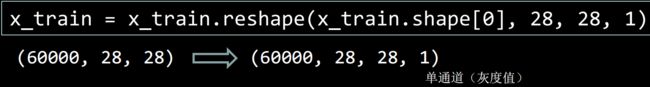

下面代码只贴出相比baseline改动的部分：

from keras.preprocessing.image import ImageDataGenerator

mnist = tf.keras.datasets.mnist
(x_train, y_train), (x_test, y_test) = mnist.load_data()
x_train, x_test = x_train / 255.0, x_test / 255.0
x_train = x_train.reshape(x_train.shape[0], 28, 28, 1)  # 给数据增加一个维度，使数据和网络结构匹配，从(60000, 28, 28)reshape为(60000, 28, 28, 1)

image_gen_train = ImageDataGenerator(
    rescale=1. / 1.,  # 如为图像，分母为255时，可归至0～1
    rotation_range=45,  # 随机45度旋转
    width_shift_range=.15,  # 宽度偏移
    height_shift_range=.15,  # 高度偏移
    horizontal_flip=False,  # 水平翻转
    zoom_range=0.5  # 将图像随机缩放 阈量50％
)
image_gen_train.fit(x_train)    # 把x_train送入数据增强操作

model.fit(image_gen_train.flow(x_train, y_train, batch_size=32), epochs=5, validation_data=(x_test, y_test), validation_freq=1)   # fit时以flow形式按照batch打包后执行训练过程

由于使用的数据为标准MNIST数据集，单纯从测试集准确率上看不出数据增强效果，需要从实际应用程序中体会

数据增强可视化

# 显示原始图像和增强后的图像
import tensorflow as tf
from matplotlib import pyplot as plt
from keras.preprocessing.image import ImageDataGenerator
import numpy as np

mnist = tf.keras.datasets.mnist
(x_train, y_train), (x_test, y_test) = mnist.load_data()
x_train = x_train.reshape(x_train.shape[0], 28, 28, 1)

image_gen_train = ImageDataGenerator(
    rescale=1. / 255,
    rotation_range=45,
    width_shift_range=.15,
    height_shift_range=.15,
    horizontal_flip=False,
    zoom_range=0.5
)
image_gen_train.fit(x_train)

print("xtrain",x_train.shape)   # (60000, 28, 28, 1)
# np.squeeze(输入的数组, axis=)  axis用于指定需要删除的维度，且必须为单维度，若为空，删除所有单维度的条目
# 返回值：数组   不会修改原数组
# 作用：从数组的形状中删除单维度条目，即把shape中为1的维度去掉
x_train_subset1 = np.squeeze(x_train[:12])
print("xtrain_subset1",x_train_subset1.shape)   # (12, 28, 28)
print("xtrain",x_train.shape)
x_train_subset2 = x_train[:12]  # 一次显示12张图片
print("xtrain_subset2",x_train_subset2.shape)    # (12, 28, 28, 1)

fig = plt.figure(figsize=(20, 2))
plt.set_cmap('gray')
# 显示原始图片
for i in range(0, len(x_train_subset1)):
    ax = fig.add_subplot(1, 12, i + 1)
    ax.imshow(x_train_subset1[i])
fig.suptitle('Subset of Original Training Images', fontsize=20)
plt.show()

# 显示增强后的图片
fig = plt.figure(figsize=(20, 2))
for x_batch in image_gen_train.flow(x_train_subset2, batch_size=12, shuffle=False):
    for i in range(0, 12):
        ax = fig.add_subplot(1, 12, i + 1)
        ax.imshow(np.squeeze(x_batch[i]))
    fig.suptitle('Augmented Images', fontsize=20)
    plt.show()
    break;

---

断点续训，存取模型

在进行神经网络训练过程中，由于一些因素导致训练无法进行，需要保存当前的训练结果下次接着训练

（一）读取模型

load_weights(路径文件名) 直接读取已有模型的参数

下面代码只贴出相比baseline改动的部分：

import os   # 为了判断保存的模型参数是否存在

checkpoint_save_path = "./checkpoint/mnist.ckpt"   # 定义存放模型的路径和文件名，命名为ckpt文件，生成ckpt文件时会同步生成索引表
if os.path.exists(checkpoint_save_path + '.index'):   # 通过判断是否存在索引表，判断是否已经保存过模型参数
    print('-------------load the model-----------------')
    model.load_weights(checkpoint_save_path)   # 若已经有了索引表，直接读取模型参数

（二）保存模型

借助TensorFlow给出的回调函数tf.keras.callbacks.ModelCheckpoint，在训练过程中保存模型的权重，并在训练结束后保存最优权重。使用回调函数可以方便地继续训练模型或加载之前训练过的模型

模板：

cp_callback = tf.keras.callbacks.ModelCheckpoint(
                filepath=路径文件名,    # 文件存储路径
                save_weights_only=True/False,   # 是否只保留模型参数
                save_best_only=True/False,   # 是否只保留最优结果
                monitor='val_loss'/'loss')   # monitor配合save_best_only可以保存最优模型，包括：训练损失最小模型、测试损失最小模型、训练准确率最高模型、测试准确率最高模型等

history = model.fit( callbacks=[cp_callback] )  # 执行训练过程时加入callbacks选项，记录到history中
# history里储存了loss和metrics结果，用于后面可视化

下面代码只贴出相比baseline改动的部分：

# 保存训练出来的模型参数，使用回调函数，返回给cp_callback
cp_callback = tf.keras.callbacks.ModelCheckpoint(filepath=checkpoint_save_path,   
                                                 save_weights_only=True,
                                                 save_best_only=True)

history = model.fit(x_train, y_train, batch_size=32, epochs=5, validation_data=(x_test, y_test), validation_freq=1, callbacks=[cp_callback])   # 在fit中加入callbacks(回调选项)，赋值给history

训练过程中出现checkpoint文件夹，里面存放的就是模型参数

再次运行，程序会加载刚才保存的模型参数：

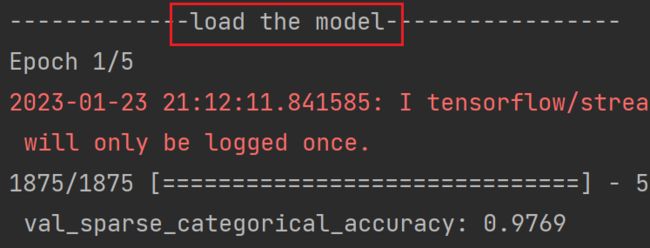
这次训练的准确率是在刚刚保存的模型基础上继续提升的

---

参数提取，把参数存入文本

（一）提取可训练参数

model.trainable_variables   # 返回模型中可训练的参数

直接print的话，很多数据会被省略号替换：

模型结构如下：

model = tf.keras.models.Sequential([
        tf.keras.layers.Flatten(),
        tf.keras.layers.Dense(128, activation='relu'),
        tf.keras.layers.Dense(10, activation='softmax')
])

模型中可训练参数有：

1. [shape=(784, 128) dtype=float32, numpy=array([[...]], dtype=float32)>

2. shape=(128,) dtype=float32, numpy=array([...],dtype=float32)>

3. shape=(128, 10) dtype=float32, numpy=array([[...]], dtype=float32)>

4. shape=(10,) dtype=float32, numpy=array([...],dtype=float32)>

（二）设置print输出格式

np.set_printoptions(
    precision=小数点后按四舍五入保留几位,
    threshold=数组元素数量少于或等于门槛值，打印全部元素；否则打印门槛值+1个元素，中间用省略号补充)

threshold = np.inf 打印全部数组元素，np.inf表示无限大

# 在断点续训的基础上添加参数提取功能
import numpy as np

np.set_printoptions(threshold=np.inf)   # 设置打印选项，打印所有内容

print(model.trainable_variables)    # 打印出所有可训练参数

file = open('./weights.txt', 'w')   # 存入文本文件
for v in model.trainable_variables:   # 用for循环把所有可训练参数存入文本
    file.write(str(v.name) + '\n')
    file.write(str(v.shape) + '\n')
    file.write(str(v.numpy()) + '\n')
file.close()

---

acc/loss可视化，查看训练效果

在model.fit执行训练过程时，同步记录了训练集loss、测试集loss、训练集准确率、测试集准确率，可以用history.history提取出来

history = model.fit(训练集数据, 训练集标签, batch_size=, epochs=, validation_split=用作测试数据的比例, validation_data=测试集, validation_freq=测试频率)   # 执行训练过程

'''
history：
训练集loss： loss
测试集loss： val_loss
训练集准确率： sparse_categorical_accuracy
测试集准确率： val_sparse_categorical_accuracy
通过history.history提取出来
'''
loss = history.history['loss']
val_loss = history.history['val_loss']
acc = history.history['sparse_categorical_accuracy']
val_acc = history.history['val_sparse_categorical_accuracy']

下面代码只贴出相比baseline改动的部分：

from matplotlib import pyplot as plt

# 显示训练集和验证集的acc和loss曲线
# 用history.history提取model.fit函数在执行训练过程中保存的：
acc = history.history['sparse_categorical_accuracy']   # 训练集准确率
val_acc = history.history['val_sparse_categorical_accuracy']   # 测试集准确率
loss = history.history['loss']   # 训练集损失函数数值
val_loss = history.history['val_loss']   # 测试集损失函数数值

plt.subplot(1, 2, 1)   # 一行两列，第一列
plt.plot(acc, label='Training Accuracy')
plt.plot(val_acc, label='Validation Accuracy')
plt.title('Training and Validation Accuracy')
plt.legend()

plt.subplot(1, 2, 2)
plt.plot(loss, label='Training Loss')
plt.plot(val_loss, label='Validation Loss')
plt.title('Training and Validation Loss')
plt.legend()
plt.show()

---

应用程序，实现给图识物