动手学数据分析—5.数据建模及模型评估
动手学数据分析—5.数据建模及模型评估
- 一、 特征工程
-
- 1.1缺失值填充
- 1.2编码分类变量
- 二、模型搭建
-
-
- tips1
- 2.1切割训练集和测试集
-
- tips2
- Q1
- 2.2 模型创建
-
- tips3
- Q2
- 2.3 输出模型预测结果
-
- tips4
- Q3
-
- 三、模型评估
-
- 3.1 交叉验证
-
- tips5
- Q4
- 3.2 混淆矩阵
-
- tips6
- Q5
- 3.3 ROC曲线
-
- tips7
- Q6
引言&复习
本章将开始数据建模。
过程将综合使用所学知识:特征工程、模型搭建与模型评估。
import pandas as pd
import numpy as np
import seaborn as sns
import matplotlib.pyplot as plt
from IPython.display import Image
%matplotlib inline
plt.rcParams['font.sans-serif'] = ['SimHei']  # 用来正常显示中文标签
plt.rcParams['axes.unicode_minus'] = False  # 用来正常显示负号
plt.rcParams['figure.figsize'] = (10, 6)  # 设置输出图片大小
# 读取训练数集
train = pd.read_csv('train.csv')
train.shape
(891, 12)
train.head()
| PassengerId | Survived | Pclass | Name | Sex | Age | SibSp | Parch | Ticket | Fare | Cabin | Embarked | |
|---|---|---|---|---|---|---|---|---|---|---|---|---|
| 0 | 1 | 0 | 3 | Braund, Mr. Owen Harris | male | 22.0 | 1 | 0 | A/5 21171 | 7.2500 | NaN | S |
| 1 | 2 | 1 | 1 | Cumings, Mrs. John Bradley (Florence Briggs Th... | female | 38.0 | 1 | 0 | PC 17599 | 71.2833 | C85 | C |
| 2 | 3 | 1 | 3 | Heikkinen, Miss. Laina | female | 26.0 | 0 | 0 | STON/O2. 3101282 | 7.9250 | NaN | S |
| 3 | 4 | 1 | 1 | Futrelle, Mrs. Jacques Heath (Lily May Peel) | female | 35.0 | 1 | 0 | 113803 | 53.1000 | C123 | S |
| 4 | 5 | 0 | 3 | Allen, Mr. William Henry | male | 35.0 | 0 | 0 | 373450 | 8.0500 | NaN | S |
一、 特征工程
本步骤旨在通过对数据进行适当处理以达到供建模使用的目的。
1.1缺失值填充
- 对分类变量缺失值:填充某个缺失值字符(NA)、用最多类别的进行填充
- 对连续变量缺失值:填充均值、中位数、众数
# 对分类变量进行填充
train['Cabin'] = train['Cabin'].fillna('NA')
train['Embarked'] = train['Embarked'].fillna('S')
# 对连续变量进行填充
train['Age'] = train['Age'].fillna(train['Age'].mean())
# 检查缺失值比例
train.isnull().mean().sort_values(ascending=False)
Embarked       0.0
Cabin          0.0
Fare           0.0
Ticket         0.0
Parch          0.0
SibSp          0.0
Age            0.0
Sex            0.0
Name           0.0
Pclass         0.0
Survived       0.0
PassengerId    0.0
dtype: float64
1.2编码分类变量
# 取出所有的输入特征
data = train[['Pclass','Sex','Age','SibSp','Parch','Fare', 'Embarked']]
# 进行虚拟变量转换
data = pd.get_dummies(data)
data.head()
| Pclass | Age | SibSp | Parch | Fare | Sex_female | Sex_male | Embarked_C | Embarked_Q | Embarked_S | |
|---|---|---|---|---|---|---|---|---|---|---|
| 0 | 3 | 22.0 | 1 | 0 | 7.2500 | 0 | 1 | 0 | 0 | 1 |
| 1 | 1 | 38.0 | 1 | 0 | 71.2833 | 1 | 0 | 1 | 0 | 0 |
| 2 | 3 | 26.0 | 0 | 0 | 7.9250 | 1 | 0 | 0 | 0 | 1 |
| 3 | 1 | 35.0 | 1 | 0 | 53.1000 | 1 | 0 | 0 | 0 | 1 |
| 4 | 3 | 35.0 | 0 | 0 | 8.0500 | 0 | 1 | 0 | 0 | 1 |
二、模型搭建
- 下一步开始选择合适模型。
- 在进行模型选择之前我们需要先知道数据集最终是进行监督学习还是无监督学习。
- 除了根据我们任务来选择模型外,还可以根据数据样本量以及特征的稀疏性来决定
- 刚开始我们会尝试使用一个基本的模型来作为其baseline,进而再训练其他模型做对比,最终选择泛化能力或性能比较好的模型
tips1
- 数据集哪些差异会导致模型在拟合数据时发生变化

2.1切割训练集和测试集
- 按比例切割训练集和测试集(一般测试集的比例有30%、25%、20%、15%和10%)
- 按目标变量分层进行等比切割
- 设置随机种子以便结果能复现
tips2
切割数据集是为了后续能评估模型泛化能力
sklearn中切割数据集的方法为train_test_split
查看函数文档可以在jupyter noteboo里面使用train_test_split?后回车即可看到
分层和随机种子在参数里寻找
Q1
- 什么情况下切割数据集的时候不用进行随机选取
from sklearn.model_selection import train_test_split
# 一般先取出X和y后再切割,有些情况会使用到未切割的,这时候X和y就可以用
X = data
y = train['Survived']
# 对数据集进行切割
X_train, X_test, y_train, y_test = train_test_split(X, y, stratify=y, random_state=0)
# 查看数据形状
X_train.shape, X_test.shape
((668, 10), (223, 10))
2.2 模型创建
- 创建基于线性模型的分类模型(逻辑回归)
- 创建基于树的分类模型(决策树、随机森林)
- 查看模型的参数,并更改参数值,观察模型变化
tips3
逻辑回归不是回归模型而是分类模型,不要与
LinearRegression混淆
随机森林其实是决策树集成为了降低决策树过拟合的情况
线性模型所在的模块为sklearn.linear_model
树模型所在的模块为sklearn.ensemble
Q2
- 为什么线性模型可以进行分类任务,背后是怎么的数学关系
- 对于多分类问题,线性模型是怎么进行分类的
from sklearn.linear_model import LogisticRegression
from sklearn.ensemble import RandomForestClassifier
# 默认参数逻辑回归模型
lr = LogisticRegression()
lr.fit(X_train, y_train)
LogisticRegression(C=1.0, class_weight=None, dual=False, fit_intercept=True,
          intercept_scaling=1, max_iter=100, multi_class='ovr', n_jobs=1,
          penalty='l2', random_state=None, solver='liblinear', tol=0.0001,
          verbose=0, warm_start=False)
# 查看训练集和测试集score值
print("Training set score: {:.2f}".format(lr.score(X_train, y_train)))
print("Testing set score: {:.2f}".format(lr.score(X_test, y_test)))
Training set score: 0.80
Testing set score: 0.78
# 调整参数后的逻辑回归模型
lr2 = LogisticRegression(C=100)
lr2.fit(X_train, y_train)
LogisticRegression(C=100, class_weight=None, dual=False, fit_intercept=True,
          intercept_scaling=1, max_iter=100, multi_class='ovr', n_jobs=1,
          penalty='l2', random_state=None, solver='liblinear', tol=0.0001,
          verbose=0, warm_start=False)
print("Training set score: {:.2f}".format(lr2.score(X_train, y_train)))
print("Testing set score: {:.2f}".format(lr2.score(X_test, y_test)))
Training set score: 0.80
Testing set score: 0.79
# 默认参数的随机森林分类模型
rfc = RandomForestClassifier()
rfc.fit(X_train, y_train)
RandomForestClassifier(bootstrap=True, class_weight=None, criterion='gini',
            max_depth=None, max_features='auto', max_leaf_nodes=None,
            min_impurity_decrease=0.0, min_impurity_split=None,
            min_samples_leaf=1, min_samples_split=2,
            min_weight_fraction_leaf=0.0, n_estimators=10, n_jobs=1,
            oob_score=False, random_state=None, verbose=0,
            warm_start=False)
print("Training set score: {:.2f}".format(rfc.score(X_train, y_train)))
print("Testing set score: {:.2f}".format(rfc.score(X_test, y_test)))
Training set score: 0.97
Testing set score: 0.82
# 调整参数后的随机森林分类模型
rfc2 = RandomForestClassifier(n_estimators=100, max_depth=5)
rfc2.fit(X_train, y_train)
RandomForestClassifier(bootstrap=True, class_weight=None, criterion='gini',
            max_depth=5, max_features='auto', max_leaf_nodes=None,
            min_impurity_decrease=0.0, min_impurity_split=None,
            min_samples_leaf=1, min_samples_split=2,
            min_weight_fraction_leaf=0.0, n_estimators=100, n_jobs=1,
            oob_score=False, random_state=None, verbose=0,
            warm_start=False)
print("Training set score: {:.2f}".format(rfc2.score(X_train, y_train)))
print("Testing set score: {:.2f}".format(rfc2.score(X_test, y_test)))
Training set score: 0.86
Testing set score: 0.83
2.3 输出模型预测结果
- 输出模型预测分类标签
- 输出不通分类标签的预测概率
tips4
一般监督模型在sklearn里面有个
predict能输出预测标签,predict_proba则可以输出标签概率
Q3
- 预测标签的概率对我们有什么帮助
# 预测标签
pred = lr.predict(X_train)
# 此时我们可以看到0和1的数组
pred[:10]
array([0, 1, 1, 1, 0, 0, 1, 0, 1, 1], dtype=int64)
# 预测标签概率
pred_proba = lr.predict_proba(X_train)
pred_proba[:10]
array([[0.62887291, 0.37112709],
       [0.14897206, 0.85102794],
       [0.47162003, 0.52837997],
       [0.20365672, 0.79634328],
       [0.86428125, 0.13571875],
       [0.9033887 , 0.0966113 ],
       [0.13829338, 0.86170662],
       [0.89516141, 0.10483859],
       [0.05735141, 0.94264859],
       [0.13593291, 0.86406709]])
三、模型评估
- 模型评估是为了知道模型的泛化能力。
- 交叉验证(cross-validation)是一种评估泛化性能的统计学方法,它比单次划分训练集和测试集的方法更加稳定、全面。
- 在交叉验证中,数据被多次划分,并且需要训练多个模型。
- 最常用的交叉验证是 k 折交叉验证(k-fold cross-validation),其中 k 是由用户指定的数字,通常取 5 或 10。
- 准确率(precision)度量的是被预测为正例的样本中有多少是真正的正例
- 召回率(recall)度量的是正类样本中有多少被预测为正类
- f-分数是准确率与召回率的调和平均
3.1 交叉验证
- 用10折交叉验证来评估逻辑回归模型
- 计算交叉验证精度的平均值

tips5
交叉验证在sklearn中的模块为
sklearn.model_selection
Q4
- k折越多的情况下会带来什么样的影响?
from sklearn.model_selection import cross_val_score
lr = LogisticRegression(C=100)
scores = cross_val_score(lr, X_train, y_train, cv=10)
# k折交叉验证分数
scores
array([0.82352941, 0.79411765, 0.80597015, 0.80597015, 0.8358209 ,
       0.88059701, 0.72727273, 0.86363636, 0.75757576, 0.71212121])
# 平均交叉验证分数
print("Average cross-validation score: {:.2f}".format(scores.mean()))
Average cross-validation score: 0.80
3.2 混淆矩阵
- 计算二分类问题的混淆矩阵
- 计算精确率、召回率以及f-分数


tips6
混淆矩阵的方法在sklearn中的
sklearn.metrics模块
混淆矩阵需要输入真实标签和预测标签
Q5
- 如果自己实现混淆矩阵的时候该注意什么问题
from sklearn.metrics import confusion_matrix
# 训练模型
lr = LogisticRegression(C=100)
lr.fit(X_train, y_train)
LogisticRegression(C=100, class_weight=None, dual=False, fit_intercept=True,
          intercept_scaling=1, max_iter=100, multi_class='ovr', n_jobs=1,
          penalty='l2', random_state=None, solver='liblinear', tol=0.0001,
          verbose=0, warm_start=False)
# 模型预测结果
pred = lr.predict(X_train)
# 混淆矩阵
confusion_matrix(y_train, pred)
array([[350,  62],
       [ 71, 185]], dtype=int64)
from sklearn.metrics import classification_report
# 精确率、召回率以及f1-score
print(classification_report(y_train, pred))
             precision    recall  f1-score   support

          0       0.83      0.85      0.84       412
          1       0.75      0.72      0.74       256

avg / total       0.80      0.80      0.80       668
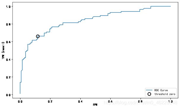
3.3 ROC曲线
- 绘制ROC曲线
tips7
ROC曲线在sklearn中的模块为
sklearn.metrics
ROC曲线下面所包围的面积越大越好
Q6
- 对于多分类问题如何绘制ROC曲线
from sklearn.metrics import roc_curve
fpr, tpr, thresholds = roc_curve(y_test, lr.decision_function(X_test))
plt.plot(fpr, tpr, label="ROC Curve")
plt.xlabel("FPR")
plt.ylabel("TPR (recall)")
# 找到最接近于0的阈值
close_zero = np.argmin(np.abs(thresholds))
plt.plot(fpr[close_zero], tpr[close_zero], 'o', markersize=10, label="threshold zero", fillstyle="none", c='k', mew=2)
plt.legend(loc=4)