YOLOv5代码阅读笔记及解析
YOLOv5代码阅读笔记
一,backbone
1,Focus
①,原理:把一个n x n x c的feature map,按步长为2,进行取值下采样。如图一所示,把原始特征图沿x轴、y轴按步长为2进行取值操作,取值后添加到通道里,然后进行一次普通卷积。
 "
"
②,代码如下:
'''
    把输入x分别从(0,0)、(1,0)、(0,1)、(1,1)开始,按步长为2取值。
    然后进行一次卷积。
'''
class Focus(nn.Module):
    # Focus wh information into c-space
    def __init__(self, c1, c2, k=1, s=1, p=None, g=1, act=True):  # ch_in, ch_out, kernel, stride, padding, groups
        super(Focus, self).__init__()
        self.conv = Conv(c1 * 4, c2, k, s, p, g, act)      # 这里输入通道变成了4倍

    def forward(self, x):  # x(b,c,w,h) -> y(b,4c,w/2,h/2)
        return self.conv(torch.cat([x[..., ::2, ::2],\
         x[..., 1::2, ::2], x[..., ::2, 1::2], x[..., 1::2, 1::2]], 1))
2,CSPDarknet
①,YOLOv5的CSP并非传统的CSP那样把输入特征分离成两份,如图二所示,传统的CSP结构是先把输入特征分离,通道数减半。
 "
"
CSPDarknet则是直接用1 x 1卷积来实现的通道缩减,如图三所示,直接对原图通过1 x 1的卷积实现通道减半,再通过concatenate把通道合并,在通过1 x 1卷积实现特征的融合。
 "
"
②,通过配置文件里的depth_multiple、width_multiple参数来控制通道数和block的数量,如原始的block为3、9、9、3, 通过block x width_multiple再取整来确定每个block的个数。如width_multiple = 0.33,则block个数为1,3,3,1,代码会详细给出解释。
3,类SPP
YOLO里的SPP并非传统的分类中的特征金字塔,传统的SPP是把特征图通过固定尺寸的池化,生成不同尺寸的特征图,如图四,把特征图依次输出为4 x 4 x 256、2 x 2 x 256、1 x 1 x 256,最后按256通道拼接后就可以放到FC中。
 "
"
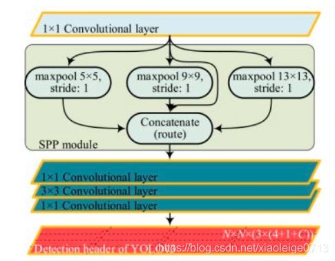
YOLO中的SPP只是借鉴了SPP的思想,如图五所示,YOLO采用统一的步长但不同尺寸的卷积核实现SPP,统一步长则代表输出的特征图尺寸一样,只是对区域的敏感性不一样,再通过concate按通道拼接后用1 x 1卷积,实现特征的融合。
 "
"
4,部分重要代码解析
①,代码整体结构
YOLOv5的backbone采用配置文件给出,所有的操作都写在配置文件里,如Conv、BottleneckCSP、SPP。在代码里构建相同名称的类,从配置文件中读取到对应的操作后就会对该操作的类实例化。整个网络结构由Model类构成,Model中调用了parse_model()函数,由该函数对配置文件进行解析后调用对应的类进行网络构建,构建后由Model实现后面处理。
②,parse_model()函数解析
parse_model()传入参数为输入通道和网络配置文件,然后对anchor个数,类别数,通道权值及block个数,及输出特征图最后一维(4 + conf + 类别数)进行了定义。同时对配置文件里的backbone和head参数放到了一起。
代码如下:
def parse_model(d, ch):  # model_dict, input_channels(3)
    logger.info('\n%3s%18s%3s%10s  %-40s%-30s' % ('', 'from', 'n', 'params', 'module', 'arguments'))
    anchors, nc, gd, gw = d['anchors'], d['nc'], d['depth_multiple'], d['width_multiple']
    na = (len(anchors[0]) // 2) if isinstance(anchors, list) else anchors  # number of anchors
    no = na * (nc + 5)  # number of outputs = anchors * (classes + 5)

    layers, save, c2 = [], [], ch[-1]  # layers, savelist, ch out
    add = d['backbone'] + d['head']
定义好以上参数后parse_model()对backbone或者head中的内容按行取出,并依次放到f, n, m, args中,如backbone的第一层[-1, 1, Focus, [64, 3]]中,f = -1代表从上一层接受特征,n = 1代表只有一个这样的操作,m = Focus代码这层要执行Focus操作,args = [64,3]代表这层输出为64维,用3*3的卷积核,步长为1。其中需要解析下 m = eval(m) if isinstance(m, str) else m 这句代码,如m是Focus,则这句就是 m = Focus,其中Focus是上面已经定义好的类,就是一个类的实例化。
代码如下:
for i, (f, n, m, args) in enumerate(d['backbone'] + d['head']):  # from, number, module, args
    m = eval(m) if isinstance(m, str) else m  # eval strings
    for j, a in enumerate(args):
        try:
            args[j] = eval(a) if isinstance(a, str) else a  # eval strings
        except:
            pass
到此该定义的值都定义完了,就需要进行网络构建了,网络先把模块要操作的个数确定,如果小于1则取1,大于1就取对应的整数,如该模块需要操作9次,但是depth_multiple: 0.33那么执行的操作个数就是9 x 0.33 = 2.97,取整后为3。再对要输出的通道数进行操作,如你本层要输出128,但是width_multiple: 0.50则输出通道为128 x 0.50 = 64。如果操作需要用到输入输出通道的,如[Conv, Bottleneck, SPP, DWConv, MixConv2d, Focus, CrossConv, BottleneckCSP, C3]则按上述操作进行,不需要则按对应的操作进行。定义好上述东西后就可以进行操作了。需要解析下ch这个玩意,它一直把c2的值存储下来,c2代表本层的输出通道,所以如果你想要找某层的输出通道就可以在ch中索引出来。
代码如下:
for i, (f, n, m, args) in enumerate(d['backbone'] + d['head']):  # from, number, module, args
    m = eval(m) if isinstance(m, str) else m  # eval strings
    for j, a in enumerate(args):
        try:
            args[j] = eval(a) if isinstance(a, str) else a  # eval strings
        except:
            pass

    n = max(round(n * gd), 1) if n > 1 else n  # depth gain
    if m in [Conv, Bottleneck, SPP, DWConv, MixConv2d, Focus, CrossConv, BottleneckCSP, C3]:
        c1, c2 = ch[f], args[0] ### 添加input的通道,以及输出通道和卷积核个数 ###

        # Normal
        # if i > 0 and args[0] != no:  # channel expansion factor
        #     ex = 1.75  # exponential (default 2.0)
        #     e = math.log(c2 / ch[1]) / math.log(2)
        #     c2 = int(ch[1] * ex ** e)
        # if m != Focus:

        c2 = make_divisible(c2 * gw, 8) if c2 != no else c2

        # Experimental
        # if i > 0 and args[0] != no:  # channel expansion factor
        #     ex = 1 + gw  # exponential (default 2.0)
        #     ch1 = 32  # ch[1]
        #     e = math.log(c2 / ch1) / math.log(2)  # level 1-n
        #     c2 = int(ch1 * ex ** e)
        # if m != Focus:
        #     c2 = make_divisible(c2, 8) if c2 != no else c2

        args = [c1, c2, *args[1:]] ### 带* 会把一些可以迭代的东西解析成一个值 ###
        if m in [BottleneckCSP, C3]:
            args.insert(2, n)
            n = 1
    elif m is nn.BatchNorm2d:
        args = [ch[f]]
    elif m is Concat:
        c2 = sum([ch[-1 if x == -1 else x + 1] for x in f])
    elif m is Detect:
        args.append([ch[x + 1] for x in f])
        if isinstance(args[1], int):  # number of anchors
            args[1] = [list(range(args[1] * 2))] * len(f)
    else:
        c2 = ch[f]

    m_ = nn.Sequential(*[m(*args) for _ in range(n)]) if n > 1 else m(*args)  # module
    t = str(m)[8:-2].replace('__main__.', '')  # module type
    np = sum([x.numel() for x in m_.parameters()])  # number params
    m_.i, m_.f, m_.type, m_.np = i, f, t, np  # attach index, 'from' index, type, number params
    logger.info('%3s%18s%3s%10.0f  %-40s%-30s' % (i, f, n, np, t, args))  # print
    save.extend(x % i for x in ([f] if isinstance(f, int) else f) if x != -1)  # append to savelist
    layers.append(m_)
    ch.append(c2)
return nn.Sequential(*layers), sorted(save)
③,本块只解析forward_once()模块
parse_model()函数构建好了网络,这就好比你在挖河,parse_model()给你挖好了沟,现在要灌水。在forward_once()中先对parse_model()构建好的网络按模块(parse_model()把网络构按索引建成了Focus,Conv,BottleneckCSP,SPP等模块,每个模块就是一层)解析,对解析到的模型进行数据套娃式据输入,通过这行代码x = m(x),把本层的输出赋值给下一层的输入,其中m代表model中存的操作,如SPP,Focus等。需要解析下这行代码x = y[m.f],这是说如果本层需要接收的数据不仅仅只有上一层,就是model中的f存的值不仅仅是-1,则通过y把需要层的数据放一起,需要对代码中y这个参数稍加解释,y中存着各个层的输出结果,可以从y中找到需要层的结果,再通过 x = m(x)进行灌水。
代码如下:
def forward_once(self, x, profile=False):
    y, dt = [], []  # outputs
    for m in self.model:
        if m.f != -1:  # if not from previous layer
            x = y[m.f] if isinstance(m.f, int) else [x if j == -1 else y[j] for j in m.f]  # from earlier layers

        if profile:
            o = thop.profile(m, inputs=(x,), verbose=False)[0] / 1E9 * 2 if thop else 0  # FLOPS
            t = time_synchronized()
            for _ in range(10):
                _ = m(x)
            dt.append((time_synchronized() - t) * 100)
            print('%10.1f%10.0f%10.1fms %-40s' % (o, m.np, dt[-1], m.type))

        x = m(x)  # run
        y.append(x if m.i in self.save else None)  # save output

    if profile:
        print('%.1fms total' % sum(dt))
    return x ### 返回检测器head的的输出 ###
二,neck - > PANET
1,PANET原理
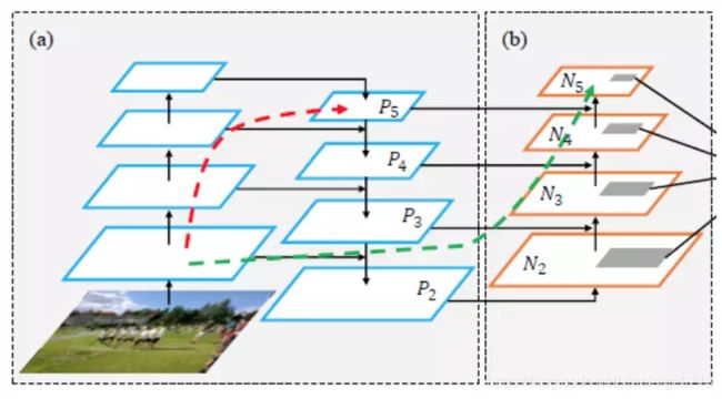
PANET原理本质来自于特征金字塔FPN,只是FPN是从上向下,PANET在FPN的基础上又从下向上进行了一波操作,具体原理如图六。
 "
"
2,PANET的代码实现
在进行代码解析前需要对YOLOv5的网络结构有详细的了解,这里盗用一下大白老师的图,网络的具体结构如图7所示,其中画黑色框的地方为拼接处。假设FPN生成的特征图用P3-P5表示,PANET拼接用F表示,依此可以在图中找到对应的PANET结构。
 "
"
从上图可以看出,要实现PANET需要从不同的层接收数据,在代码中需要实现从指定的层接收数据。model会把f(代表在构造网络时的第几层)参数存进了,如需要P5和block4拼接的时候配置文件为[[-1, 6], 1, Concat, [1]],其中f为[-1,6],代表从上一层和第六层的输出进行Concate,[1]代表在第一维。其他实现同理。
代码如下:
for m in self.model:
            if m.f != -1:  # if not from previous layer
                x = y[m.f] if isinstance(m.f, int) else [x if j == -1 else y[j] for j in m.f]  # from earlier layers
y.append(x if m.i in self.save else None)  # save output
三,head
经过PANET后生成的特征图,再经过卷积后生成尺寸和通道为b x anchor x w x h x (4+1+类别数)的特征图,用于后面的loss计算,类似于YOLOv3没啥新颖的地方。
四,loss计算
1,原理
YOLO的原理和其他单阶段的检测的原理不太一样,这里对YOLOv5中loss计算详细介绍下。首先YOLOv5会对各个target分配负责它的anchor,然后用这些anchor按target的中心点、w、h、类别去回归和分类。
分配规则为:先对输出的各个head按层(原代码中为三层)匹配anchor。如我们生成的一层head为64 x 3 x 80 x 80 x 9,这时候YOLOv5会把target中的x,y,w,h分别乘80。把target化成相对于当前feature map的尺寸。这时候x,y会落在当前feature map的某个cell里,这个cell就负责检测这个target。但是每个cell有三个不同尺寸的anchor,这时候的YOLOv5设置了过滤条件,需要目标的长宽和target的长宽比在0.25和4之间(0.25
2,built_target()代码
built_target()函数是上述原理的详细实现,也是YOLOv5的精髓。下面将会对本部分代码仔细解析。下面代码中,先从model里获取head的输出结果,然后获取了anchor数(3个)及target个数。ai = torch.arange(na, device=targets.device).float().view(na, 1).repeat(1, nt) 通过这行代码对taget复制了三份,从1 x target x 6 (6:图像序号,类别,x,y,w,h)变成了3 x target x 6 ,同时又通过targets = torch.cat((targets.repeat(na, 1, 1),
ai[:,:, None]), 2) 这行代码变成了3 x target x 7,第7维添加了0,1,2这三个值,这代表着这个target由cell里的0,1,2三个anchor里的哪个负责。
代码如下:
det = model.module.model[-1] if is_parallel(model) else model.model[-1]  ### 获取model里的detect层,里面有对应的参数 ###
    na, nt = det.na, targets.shape[0]  ### number of anchors, targets ###
    tcls, tbox, indices, anch = [], [], [], []
    gain = torch.ones(7, device=targets.device)  # normalized to gridspace gain
    ai = torch.arange(na, device=targets.device).float().view(na, 1).repeat(1, nt)  # same as .repeat_interleave(nt)
    kk = targets.repeat(na, 1, 1) ### 对原始数在0维复制三份,复制后会得到3*106*6尺寸 ###
    dd = ai[:, :, None]
    targets = torch.cat((targets.repeat(na, 1, 1), ai[:, :, None]), 2)  ### append anchor indices 3*106*7,7分别为索引,label,bbx,和复制的第几个值 ###

    g = 0.5  # bias

    off = torch.tensor([[0, 0],
                        [1, 0], [0, 1], [-1, 0], [0, -1],  # j,k,l,m
                        # [1, 1], [1, -1], [-1, 1], [-1, -1],  # jk,jm,lk,lm
                        ], device=targets.device).float() * g  # offsets
下面代码是对target筛选。先是获取本层的anchor数,然后对gain这个list中2:6维换成当前特征图的w,h。t = targets x gain经过这段代码,target中的目标就换算成了相对于当前特征图大小了,如果有目标则通过下面三行代码把target/anchor约束到0.25到4中。再把t中不符合条件的滤掉,这时候就完成了当前特征层对target的筛选。
代码如下:
r = t[:, :, 4:6] / anchors[:, None]
test = torch.max(r, 1. / r)
j = torch.max(r, 1. / r).max(2)[0] < model.hyp['anchor_t']
 for i in range(det.nl):  ### nl:number of layers ###
    anchors = det.anchors[i] ### 3个head, 每个head为3个anchor,每个anchor为w*h ###
    gain[2:6] = torch.tensor(p[i].shape)[[3, 2, 3, 2]]  # xyxy gain  p: 64*3*80*80*9 64*3*40*40*9 64*3*20*20*9
    ### gain 保留了每个p层的预测尺寸 ###

    # Match targets to anchors
    t = targets * gain ### 获取了原目标相对特征图的坐标 3*106*7 ###
    if nt: ### 如果有目标 ###
        # Matches
        r = t[:, :, 4:6] / anchors[:, None]  ### ps:每个GT/对应的anchor,3*xx*7/3*2 是3对应相除,实质为106*2/2,对应特征图的GT尺寸/对应层的anchor尺寸,得到对应特征图GT相对于anchor的ratio ###
        test = torch.max(r, 1. / r)
        j = torch.max(r, 1. / r).max(2)[0] < model.hyp['anchor_t']  ### 限定GT/ahchor or anchor/GT 在四倍内 ###
        # j = wh_iou(anchors, t[:, 4:6]) > model.hyp['iou_t']  # iou(3,n)=wh_iou(anchors(3,2), gwh(n,2))
        t = t[j]  ### 过滤后剩余的target数,剩余24*7 ###
本部分代码为扩充正样本。gxy为target中的x,y相对本层feature map的位置,或者这样理解,x,y向上取整后为负责这个target的cell的左上角坐标。gxi为特征图尺寸 - x,y。这样把中心坐标的位置反过来,其实我感觉这里真的蠢,直接用1- (gxy % 1)不就行了吗,不知道作者为啥这样写。反正是指得到当前target中心点相对于cell中心点是偏向哪里,比如偏向于左下方,则经过offsets = (torch.zeros_like(gxy)[None] + off[:, None])[j]这行代码后会把和这个cell相邻的左边和下面的cell也当成负责target的cell。其实就是把target的中心坐标±0.5的问题,把target的中心坐标偏移了一点,wh不变,依次多出来了两个target。
代码如下:
gxy = t[:, 2:4]  ### grid xy,t为尺寸*归一化后的值,gxy为目标在特征图长宽 ###
gxi = gain[[2, 3]] - gxy  ### gain为原始值,gxy为t中取值, inverse ###
j, k = ((gxy % 1. < g) & (gxy > 1.)).T
l, m = ((gxi % 1. < g) & (gxi > 1.)).T
j = torch.stack((torch.ones_like(j), j, k, l, m))
t = t.repeat((5, 1, 1))[j]
offsets = (torch.zeros_like(gxy)[None] + off[:, None])[j] ### 经过操作后,实现了±0.5的操作 ###
本部分代码为anchor和target匹配。先从t中把image的索引和类别取出。gxy为x,y。gwh为w,h。gij为负责这个target的cell左上角坐标。gi,gj为取出这个值。a为第几个anchor负责这个target的索引。indices里存里图像索引,anchor索引,负责target的cell。tbox存了xy相对于负责它的cell左上角的距离,和target相对于当前特征图的w,h。anchor为负责的anchor(如第二个anchor负责,则值为1),tcls为类别。
代码如下:
b, c = t[:, :2].long().T  # image, class
gxy = t[:, 2:4]  # grid xy
gwh = t[:, 4:6]  # grid wh
gij = (gxy - offsets).long() ### ±0.5后会出现在各个相邻的cell中,取.long后会是各个负责target的cell的左上角坐标 ###
gi, gj = gij.T  # grid xy indices

# Append
a = t[:, 6].long()  # anchor indices
indices.append((b, a, gj.clamp_(0, gain[3] - 1), gi.clamp_(0, gain[2] - 1)))  ### image, anchor, grid indices(在哪个cell负责) ###
tbox.append(torch.cat((gxy - gij, gwh), 1))  ### gxy - gij 为扩展target的中心点,gwh为目标宽高 ###
anch.append(anchors[a])  # anchors
tcls.append(c)  # class
3,预处理代码
下面代码是从整个pred中挑选target对应的部分用于loss计算,ps = pi[b, a, gj, gi] 只把b,a,gj,gi索引的预测挑出来。
代码如下:
for i, pi in enumerate(p):  # layer index, layer predictions
    b, a, gj, gi = indices[i]  # image, anchor, gridy, gridx
    tobj = torch.zeros_like(pi[..., 0], device=device)  # target obj

    n = b.shape[0]  # number of targets
    if n:
        nt += n  # cumulative targets
        ps = pi[b, a, gj, gi]  ### 从预测值中按target取第几个图像,第几个anchor,第几个cell,ps为target*9 ###
3,分类loss
分类loss使用二分类交叉熵,把target类别和pred类别进行交叉熵计算。
if model.nc > 1:  # cls loss (only if multiple classes)
    t = torch.full_like(ps[:, 5:], cn, device=device)  ### t为72*4的0 ###
    t[range(n), tcls[i]] = cp ### 在72*4中,tcls[i]中的类为1,其余为0 ###
    lcls += BCEcls(ps[:, 5:], t)  ### 预测值和真值做二进制交叉熵,但是只计算了带有GT的预测值,不带预测值的不计算 ###
4,回归loss
回归loss中有部分不解。 pxy = ps[:, :2].sigmoid() * 2. - 0.5 为什么 x 2 - 0.5?
pwh = (ps[:, 2:4].sigmoid() * 2) ** 2 * anchors[i]为什么 x 2后平方?
其他的就是把target和pred计算一个CIOU,让anchor回归到target的x,y,w,h。
pxy = ps[:, :2].sigmoid() * 2. - 0.5 ### 预测值的xy ###
pwh = (ps[:, 2:4].sigmoid() * 2) ** 2 * anchors[i] ### 预测值的wh ###
pbox = torch.cat((pxy, pwh), 1)  ### 经过修正后的预测框 ###
iou = bbox_iou(pbox.T, tbox[i], x1y1x2y2=False, CIoU=True)  # iou(prediction, target)
lbox += (1.0 - iou).mean()  # iou loss
5,置信度loss
置信度loss比较有意思,tobj刚开始都是0,然后通过这行代码tobj[b, a, gj, gi] = (1.0 - model.gr) + model.gr * iou.detach().clamp(0).type(tobj.dtype) # iou ratio对有目标的cell和anchor赋值IoU的值和1(代表有目标),其他的没有目标的都是0,代表IoU0和没有目标,最后通过这行代码lobj += BCEobj(pi[…, 4], tobj) * balance[i] ### tobj 为cell和target的IoU大小 ###,拿这个tobj和整体的预测值进行二分类交叉熵。所以整个loss里只有置信度计算了负样本,分类和回归都是只对正样本计算loss。
if n:
    nt += n  # cumulative targets
    ps = pi[b, a, gj, gi]  ### 从预测值中按target取第几个图像,第几个anchor,第几个cell,ps为target*9 ###

    ### Regression 只回归有索引成功的目标 ###
    pxy = ps[:, :2].sigmoid() * 2. - 0.5 ### 预测值的xy ###
    pwh = (ps[:, 2:4].sigmoid() * 2) ** 2 * anchors[i] ### 预测值的wh ###
    pbox = torch.cat((pxy, pwh), 1)  ### 经过修正后的预测框 ###
    iou = bbox_iou(pbox.T, tbox[i], x1y1x2y2=False, CIoU=True)  # iou(prediction, target)
    lbox += (1.0 - iou).mean()  # iou loss

    # Objectness
    tobj[b, a, gj, gi] = (1.0 - model.gr) + model.gr * iou.detach().clamp(0).type(tobj.dtype)  # iou ratio

    # Classification
    if model.nc > 1:  # cls loss (only if multiple classes)
        t = torch.full_like(ps[:, 5:], cn, device=device)  ### t为72*4的0 ###
        t[range(n), tcls[i]] = cp ### 在72*4中,tcls[i]中的类为1,其余为0 ###
        lcls += BCEcls(ps[:, 5:], t)  ### 预测值和真值做二进制交叉熵,但是只计算了带有GT的预测值,不带预测值的不计算 ###

    # Append targets to text file
    # with open('targets.txt', 'a') as file:
    #     [file.write('%11.5g ' * 4 % tuple(x) + '\n') for x in torch.cat((txy[i], twh[i]), 1)]

lobj += BCEobj(pi[..., 4], tobj) * balance[i]  ### tobj 为cell和target的IoU大小 ###
五,后处理(和其他检测方法一样,不做解析)
1,nms
2,mAP计算