R实战| PCA、tSNE、UMAP三种降维方法在R中的实现

降维

在组学分析中，一般通过降维算法得到低纬度如二维或三维的新坐标数据，再结合可视化技术去展示样本的在新坐标的空间分布，接着加上统计检验结果证实整体组学水平上组间的差异性。降维算法有基于线性模型的PCA，也有基于非线性的tSNE和UMAP等方法。

示例数据和代码领取

详见：R实战| PCA、tSNE、UMAP三种降维方法在R中的实现

PCA

主成分分析（Principal Component Analysis，PCA）是最常用的无监督学习方法。

rm(list = ls())
library(tidyverse)
library(broom)
library(palmerpenguins)

# 示例数据
penguins <- penguins %>%
  drop_na() %>%
  select(-year)
head(penguins)

# 使用prcomp()进行PCA
# PCA前对数值型数据进行标准化
pca_fit <- penguins %>%
  select(where(is.numeric)) %>%
  scale() %>%
  prcomp()
# 查看成分重要性
summary(pca_fit)

# 可视化PC1和PC2
pca_fit %>%
  augment(penguins) %>%
  rename_at(vars(starts_with(".fitted")),
            list(~str_replace(.,".fitted",""))) %>%
  ggplot(aes(x=PC1, 
             y=PC2,
             color=species,
             shape=sex))+
  geom_point()

PCA plot: PC1 vs PC2

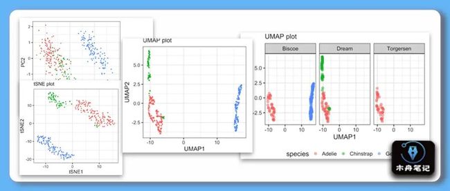
UMAP

数据预处理

## UMAP
rm(list = ls())
library(tidyverse)
library(palmerpenguins)
#install.packages("umap")
library(umap)
theme_set(theme_bw(18))

penguins <- penguins %>% 
  drop_na() %>%
  select(-year)%>%
  mutate(ID=row_number()) 

penguins_meta <- penguins %>%
  select(ID, species, island, sex)

使用umap包进行umap分析

set.seed(142)
umap_fit <- penguins %>%
  select(where(is.numeric)) %>%
  column_to_rownames("ID") %>%
  scale() %>% 
  umap()

umap_df <- umap_fit$layout %>%
  as.data.frame()%>%
  rename(UMAP1="V1",
         UMAP2="V2") %>%
  mutate(ID=row_number())%>%
  inner_join(penguins_meta, by="ID")
umap_df %>% head()

可视化

# 可视化
umap_df %>%
  ggplot(aes(x = UMAP1, 
             y = UMAP2, 
             color = species,
             shape = sex))+
  geom_point()+
  labs(x = "UMAP1",
       y = "UMAP2",
       subtitle = "UMAP plot")

UMAP plot in R: Example 1

# 分面
umap_df %>%
  ggplot(aes(x = UMAP1, 
             y = UMAP2,
             color = species)) +
  geom_point(size=3, alpha=0.5)+
  facet_wrap(~island)+
  labs(x = "UMAP1",
       y = "UMAP2",
       subtitle="UMAP plot")+
  theme(legend.position="bottom")

UMAP plot in R: Example 2

# 圈出异常样本
library(ggforce)
umap_df %>%
  ggplot(aes(x = UMAP1,
             y = UMAP2, 
             color = species,
             shape = sex)) +
  geom_point() +
  labs(x = "UMAP1",
       y = "UMAP2",
       subtitle="UMAP plot") +
  geom_circle(aes(x0 = -5, y0 = -3.8, r = 0.65), 
              color = "green",
              inherit.aes = FALSE)

UMAP Plot to Identify Potential sample mix-ups

tSNE

数据预处理

## tSNE
rm(list = ls())
library(tidyverse)
library(palmerpenguins)
library(Rtsne)
theme_set(theme_bw(18))

penguins <- penguins %>% 
  drop_na() %>%
  select(-year)%>%
  mutate(ID=row_number())

penguins_meta <- penguins %>%
  select(ID,species,island,sex)

使用Rtsne 包进行tSNE 分析

set.seed(142)
tSNE_fit <- penguins %>%
  select(where(is.numeric)) %>%
  column_to_rownames("ID") %>%
  scale() %>% 
  Rtsne()

tSNE_df <- tSNE_fit$Y %>% 
  as.data.frame() %>%
  rename(tSNE1="V1",
         tSNE2="V2") %>%
  mutate(ID=row_number())

tSNE_df <- tSNE_df %>%
  inner_join(penguins_meta, by="ID")

tSNE_df %>% head()

可视化

tSNE_df %>%
  ggplot(aes(x = tSNE1, 
             y = tSNE2,
             color = species,
             shape = sex))+
  geom_point()+
  theme(legend.position="bottom")

tSNE Plot

参考

1. How To Make tSNE plot in R - Data Viz with Python and R (datavizpyr.com)

2. How to make UMAP plot in R - Data Viz with Python and R (datavizpyr.com)

3. How To Make PCA Plot with R - Data Viz with Python and R (datavizpyr.com)

往期内容

1. CNS图表复现|生信分析|R绘图 资源分享&讨论群！

2. 组学生信| Front Immunol |基于血清蛋白质组早期诊断标志筛选的简单套路

---

木舟笔记矩阵