Lesson12---人工神经网络(1)
12.1 神经元与感知机
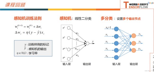
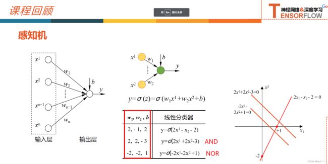
12.1.1 感知机
感知机: 1957, Fank Rosenblatt

由两层神经元组成,可以简化为右边这种,输入通常不参与计算,不计入神经网络的层数,因此感知机是一个单层神经网络
- 感知机
训练法则(Perceptron Training Rule)

- 使用感知机训练法则,能够根据训练样本的标签值和感知机输出之间的误差,来自动的调整权值,具备学习能力
- 第一个用算法来精确定义的神经网络模型
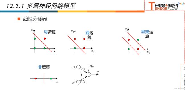
- 线性二分类的分类器,分类决策边界为直线(2v)、平面(3v)、超平面(多维)
- 感知机算法存在多个解,受到权值向量初始值,错误样本顺序的影响
- 对于非线性可分得数据集,感知机训练法则无法收敛,迭代结果会一直震荡。
- 为了克服非线性数据集无法收敛的情况,提出了delta法则
12.1.2 Delta法则
- Delta法则:使用梯度下降法,找到能够最佳拟合训练样本集的权向量
- 逻辑回归可以看作是最简单的单层神经网络,单个感知机只有一个输出节点,只能实现二分类问题
12.2 实例: 单层神经网络实现鸢尾花分类
- 这里我们使用神经网络的思想来实现对鸢尾花的分类,这个程序的实现过程和sofmax回归几乎是完全一样的,我们只是从设计和实现神经网络的角度重新描述这个过程
12.2.1 神经网络的设计
- 设计
- 首先设计 神经网络的结构,确定神经网络有几层,每层中有几个节点,节点间是如何连接的。
- 使用什么激活函数
- 使用什么损失函数
- 选择
- 选择单层前馈型神经网络的结构,实现对鸢尾花的分类,输入节点的个数由属性的个数决定,输出曾节点个数由分类类别的个数决定

- 因为是分类问题,所以选择softmax函数作为激活函数,标签值使用独热编码来表示
- 使用交叉熵损失函数来计算误差
12.2.2 神经网络的实现
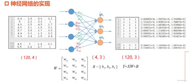
前面为了简化编程,将B融入w,为
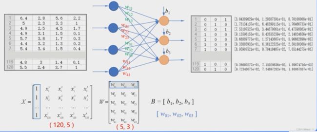
在本节中,我们将W和b分离开来,单独表示,这是考虑到后面实现多层神经网络时,编程更加直观
12.2.3 神经网络的实现的重要函数
12.2.3.1 softmax函数
tf.nn.softmax()
对于 Y = X W + B Y=XW+B Y=XW+B
tf.nn.softmax(tf.matmul(X_train,W)+b)
12.2.3.2 独热编码-tf.one_hot()
tf.one_hot(indices,depth)
- indices:要求是一个整数
- depth:独热编码的深度
对于该例鸢尾花数据
tf.one_hot(tf.constant(y_test,dtype=tf.int32),3)
12.2.3.3 交叉熵损失函数-tf.keras.losses.categorical_crossentropy()
使用其自带的来实现
tf.keras.losses.categorical_crossentropy(y_true,y_pred)
- y_true :表示独热编码的标签值
- y_pred:softmax函数的输出
- 该函数的结果时一个一维张量,其中的每一个元素是每个样本的交叉熵损失,使用求平均值函数得到平均交叉熵损失
tf.reduce_mean(tf.keras.losses.categorical_crossentropy(y_true=Y_train,y_pred=PRED_train))
12.2.4 完整的程序实现
12.2.4.1 导入库
- InternalError: Bias GEMM launch failed报错解决如下
# 1 导入库
import tensorflow as tf
print("TensorFlow version: ", tf.__version__)

import pandas as pd
import numpy as np
import matplotlib.pyplot as plt

# 在使用GPU版本的Tensorflow训练模型时,有时候会遇到显存分配的错误
# InternalError: Bias GEMM launch failed
# 这是在调用GPU运行程序时,GPU的显存空间不足引起的,为了避免这个错误,可以对GPU的使用模式进行设置
gpus = tf.config.experimental.list_physical_devices('GPU')# 这是列出当前系统中的所有GPU,放在列表gpus中
# 使用第一块gpu,所以是gpus[0],把它设置为memory_growth模式,允许内存增长也就是说在程序运行过程中,根据需要为TensoFlow进程分配显存
# 如果系统中有多个GPU,可以使用循环语句把它们都设置成为true模式
tf.config.experimental.set_memory_growth(gpus[0], True)
12.2.4.2 加载数据
TRAIN_URL = "http://download.tensorflow.org/data/iris_training.csv"
TEST_URL = "http://download.tensorflow.org/data/iris_test.csv"

train_path = tf.keras.utils.get_file(TRAIN_URL.split('/')[-1],TRAIN_URL)
test_path = tf.keras.utils.get_file(TEST_URL.split('/')[-1],TEST_URL)

df_iris_train = pd.read_csv(train_path, header=0)
df_iris_test = pd.read_csv(test_path, header=0)

iris_train = np.array(df_iris_train) # (120,5)
iris_train = np.array(df_iris_test) # (30 5)
12.2.4.3 数据预处理
# 3 数据预处理
x_train = iris_train[:,0:4] # (120,4)
y_train = iris_train[:,4] # (120,)

x_test = iris_test[:,0:4] # (30,4)
y_test = iris_test[:,4] # (30,)
# 以上4个数据都是64位浮点数('float64')

# 对属性值进行标准化处理,使它均值为0
x_train = x_train - np.mean(x_train, axis=0)
x_test = x_test - np.mean(x_test, axis=0)

X_train = tf.cast(x_train,tf.float32)
Y_train = tf.one_hot(tf.costant(y_train,dtype=tf.int32),3)

X_test = tf.cast(x_test,tf.float32)
Y_test = tf.one_hot(tf.constant(y_test,dtype=tf.int32),3)
# 以上4个数据都是float32形式的tensorflow的张量
12.2.4.4 设置超参数和显示间隔
# 4 设置超参数和显示间隔
learn_rate = 0.5
iter = 50

display_step = 10
12.2.4.5 设置模型参数初始值
# 5 设置模型参数初始值
np.random.seed(612)
W = tf.Variable(np.random.randn(4,3),dtype=tf.float32)# W为4行3列的二维张量,取正态分布的随机值
B = tf.Variable(np.zeros([3]),dtype=tf.float32) # B为长度为3的一维张量,在神经网络中,初始化为0
12.2.4.6 训练模型
# 6 训练模型

# 准确率
acc_train=[]
acc_test=[]
# 交叉熵损失
cce_train=[]
cce_test=[]

for  i in range(0,iter+1):
    with tf.GradientTape() as tape:
        PRED_train = tf.nn.softmax(tf.matmul(X_train,W)+B) # 激活函数为S函数
        Loss_train = tf.reduce_mean(tf.keras.losses.categorical_crossentropy(y_true=Y_train,y_pred=PRED_train)) # 训练集的交叉熵损失

    PRED_test = tf.nn.softmax(tf.matmul(X_test,W)+B)
    Loss_test = tf.reduce_mean(tf.keras.losses.categorical_crossentropy(y_true=Y_test,y_pred=PRED_test)) # 测试集的交叉熵损失

    accuracy_train = tf.reduce_mean(tf.cast(tf.equal(tf.argmax(PRED_train.numpy(),axis=1),y_train),tf.float32))
    accuracy_test = tf.reduce_mean(tf.cast(tf.equal(tf.argmax(PRED_test.numpy(),axis=1),y_test),tf.float32))

    acc_train.append(accuracy_train)
    acc_test.append(accuracy_test)
    cce_train.append(Loss_train)
    cce_test.append(Loss_test)

    grads = tape.gradient(Loss_train,[W,B])
    W.assign_sub(learn_rate*grads[0])
    B.assign_sub(learn_rate*grads[1])

    if i % display_step == 0:
        print("i: %i,TrainAcc:%f, TrainLoss:%f,TestAcc:%f,TestLoss:%f" % (i,accuracy_train,Loss_train,accuracy_test,Loss_test))
运行结果:
i: 0,TrainAcc:0.333333, TrainLoss:2.066978,TestAcc:0.266667,TestLoss:1.880856
i: 10,TrainAcc:0.875000, TrainLoss:0.339410,TestAcc:0.866667,TestLoss:0.461705
i: 20,TrainAcc:0.875000, TrainLoss:0.279647,TestAcc:0.866667,TestLoss:0.368414
i: 30,TrainAcc:0.916667, TrainLoss:0.245924,TestAcc:0.933333,TestLoss:0.314814
i: 40,TrainAcc:0.933333, TrainLoss:0.222922,TestAcc:0.933333,TestLoss:0.278643
i: 50,TrainAcc:0.933333, TrainLoss:0.205636,TestAcc:0.966667,TestLoss:0.251937
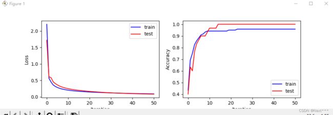
12.2.4.7 可视化
# 7 结果可视化
plt.figure(figsize=(10,3))

plt.subplot(121)
plt.plot(cce_train,c='b',label="train")
plt.plot(cce_test,c='r',label="test")
plt.xlabel("Iteration")
plt.ylabel("Loss")
plt.legend()

plt.subplot(122)
plt.plot(acc_train,c='b',label="train")
plt.plot(acc_test,c='r',label="test")
plt.xlabel("Iteration")
plt.ylabel("Accuracy")
plt.legend()

plt.show()
输出结果:

12.2.4.8 完整程序
# 1 导入库
from sys import displayhook
import tensorflow as tf
print("TensorFlow version: ", tf.__version__)

import pandas as pd
import numpy as np
import matplotlib.pyplot as plt

# 在使用GPU版本的Tensorflow训练模型时,有时候会遇到显存分配的错误
# InternalError: Bias GEMM launch failed
# 这是在调用GPU运行程序时,GPU的显存空间不足引起的,为了避免这个错误,可以对GPU的使用模式进行设置
gpus = tf.config.experimental.list_physical_devices('GPU')# 这是列出当前系统中的所有GPU,放在列表gpus中
# 使用第一块gpu,所以是gpus[0],把它设置为memory_growth模式,允许内存增长也就是说在程序运行过程中,根据需要为TensoFlow进程分配显存
# 如果系统中有多个GPU,可以使用循环语句把它们都设置成为true模式
tf.config.experimental.set_memory_growth(gpus[0], True)

# 2 加载数据

TRAIN_URL = "http://download.tensorflow.org/data/iris_training.csv"
TEST_URL = "http://download.tensorflow.org/data/iris_test.csv"

train_path = tf.keras.utils.get_file(TRAIN_URL.split('/')[-1],TRAIN_URL)
test_path = tf.keras.utils.get_file(TEST_URL.split('/')[-1],TEST_URL)

df_iris_train = pd.read_csv(train_path, header=0)
df_iris_test = pd.read_csv(test_path, header=0)

iris_train = np.array(df_iris_train) # (120,5)
iris_test = np.array(df_iris_test) # (30 5)


# 3 数据预处理
x_train = iris_train[:,0:4] # (120,4)
y_train = iris_train[:,4] # (120,)

x_test = iris_test[:,0:4] # (30,4)
y_test = iris_test[:,4] # (30,)
# 以上4个数据都是64位浮点数('float64')

# 对属性值进行标准化处理,使它均值为0
x_train = x_train - np.mean(x_train, axis=0)
x_test = x_test - np.mean(x_test, axis=0)

X_train = tf.cast(x_train,tf.float32)
Y_train = tf.one_hot(tf.constant(y_train,dtype=tf.int32),3)

X_test = tf.cast(x_test,tf.float32)
Y_test = tf.one_hot(tf.constant(y_test,dtype=tf.int32),3)
# 以上4个数据都是float32形式的tensorflow的张量

# 4 设置超参数和显示间隔
learn_rate = 0.5
iter = 50

display_step = 10

# 5 设置模型参数初始值
np.random.seed(612)
W = tf.Variable(np.random.randn(4,3),dtype=tf.float32)# W为4行3列的二维张量,取正态分布的随机值
B = tf.Variable(np.zeros([3]),dtype=tf.float32) # B为长度为3的一维张量,在神经网络中,初始化为0

# 6 训练模型

# 准确率
acc_train=[]
acc_test=[]
# 交叉熵损失
cce_train=[]
cce_test=[]

for  i in range(0,iter+1):
    with tf.GradientTape() as tape:
        PRED_train = tf.nn.softmax(tf.matmul(X_train,W)+B) # 激活函数为S函数
        Loss_train = tf.reduce_mean(tf.keras.losses.categorical_crossentropy(y_true=Y_train,y_pred=PRED_train)) # 训练集的交叉熵损失

    PRED_test = tf.nn.softmax(tf.matmul(X_test,W)+B)
    Loss_test = tf.reduce_mean(tf.keras.losses.categorical_crossentropy(y_true=Y_test,y_pred=PRED_test)) # 测试集的交叉熵损失

    accuracy_train = tf.reduce_mean(tf.cast(tf.equal(tf.argmax(PRED_train.numpy(),axis=1),y_train),tf.float32))
    accuracy_test = tf.reduce_mean(tf.cast(tf.equal(tf.argmax(PRED_test.numpy(),axis=1),y_test),tf.float32))

    acc_train.append(accuracy_train)
    acc_test.append(accuracy_test)
    cce_train.append(Loss_train)
    cce_test.append(Loss_test)

    grads = tape.gradient(Loss_train,[W,B])
    W.assign_sub(learn_rate*grads[0])
    B.assign_sub(learn_rate*grads[1])

    if i % display_step == 0:
        print("i: %i,TrainAcc:%f, TrainLoss:%f,TestAcc:%f,TestLoss:%f" % (i,accuracy_train,Loss_train,accuracy_test,Loss_test))

# 7 结果可视化
plt.figure(figsize=(10,3))

plt.subplot(121)
plt.plot(cce_train,c='b',label="train")
plt.plot(cce_test,c='r',label="test")
plt.xlabel("Iteration")
plt.ylabel("Loss")
plt.legend()

plt.subplot(122)
plt.plot(acc_train,c='b',label="train")
plt.plot(acc_test,c='r',label="test")
plt.xlabel("Iteration")
plt.ylabel("Accuracy")
plt.legend()

plt.show()
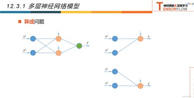
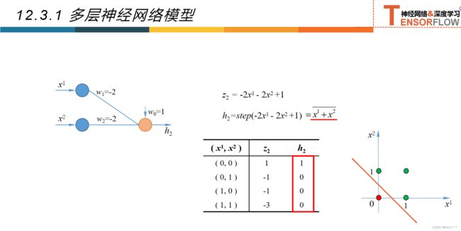
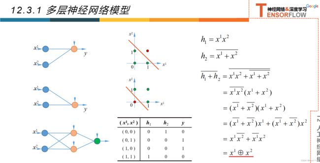
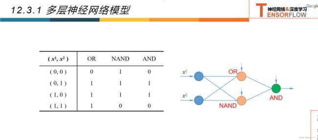
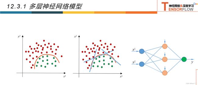
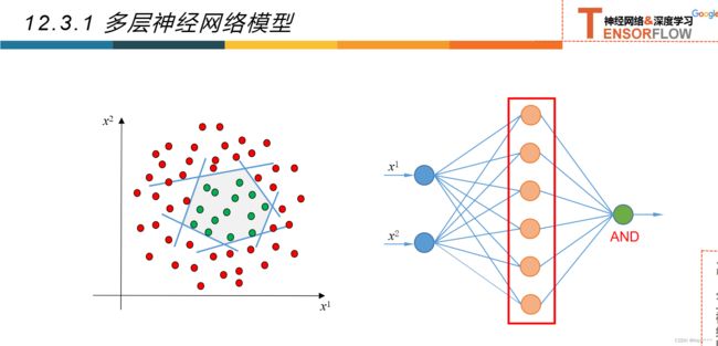
12.3多层神经网络

12.3.1多层神经网络


12.3.2超参数和验证集


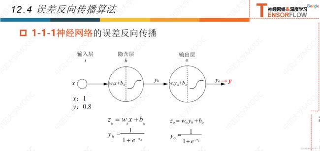
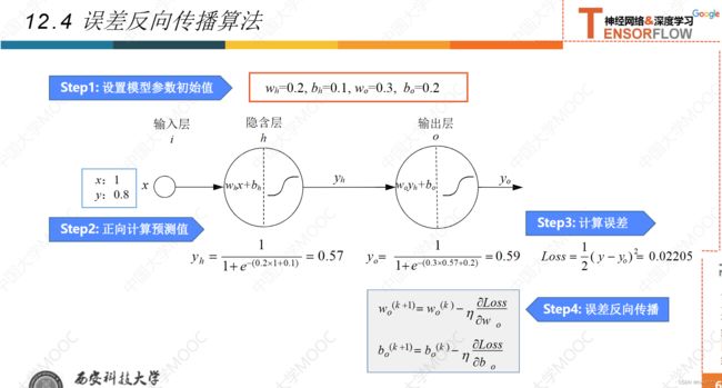
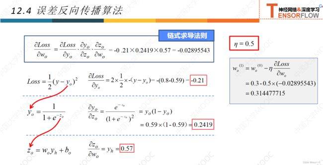
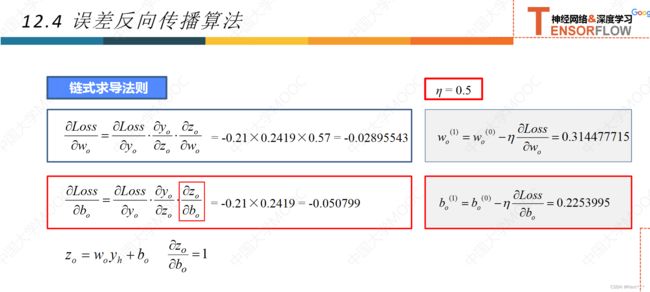
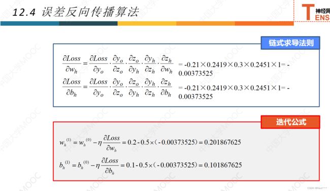
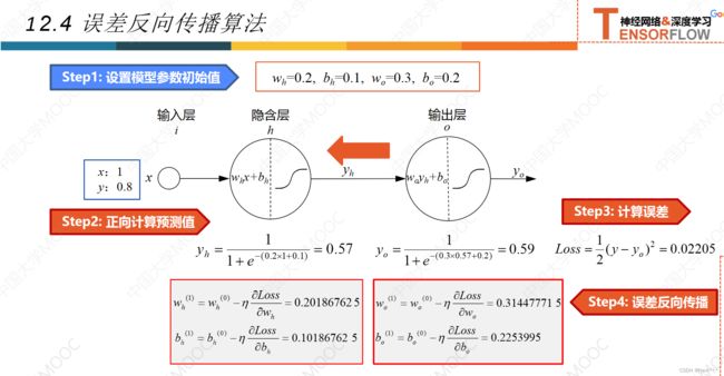
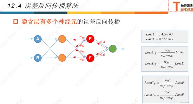
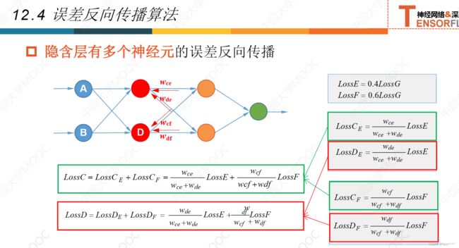
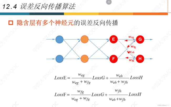
12.4误差反向传播法


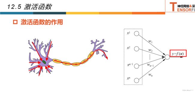
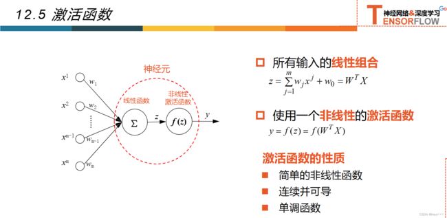
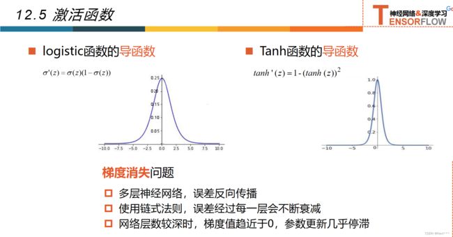
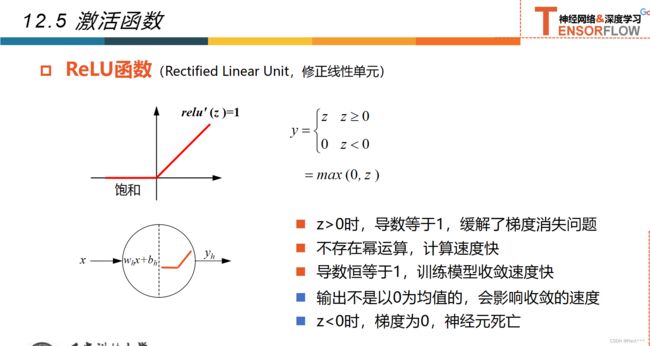
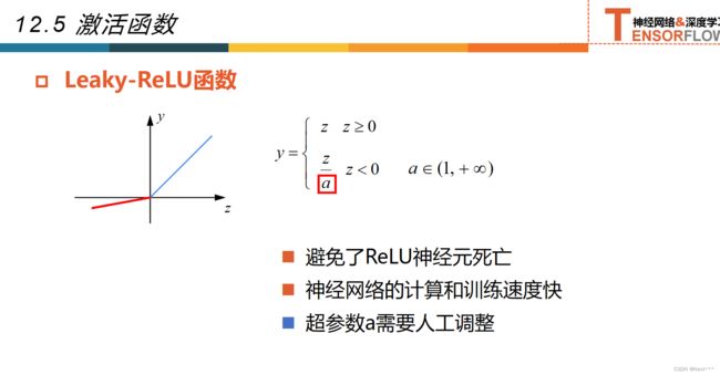
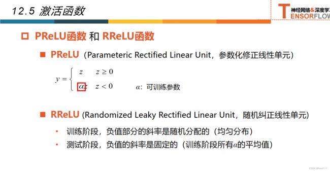
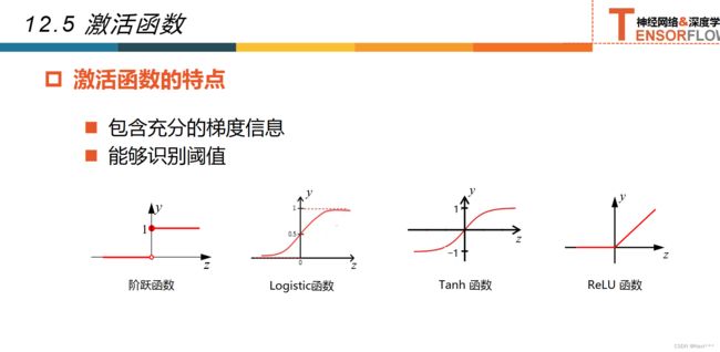
12.5激活函数


12.6 实例:多层神经网络实现鸢尾花分类

# 1 导入库
from sys import displayhook
import tensorflow as tf
print("TensorFlow version: ", tf.__version__)

import pandas as pd
import numpy as np
import matplotlib.pyplot as plt

# 在使用GPU版本的Tensorflow训练模型时,有时候会遇到显存分配的错误
# InternalError: Bias GEMM launch failed
# 这是在调用GPU运行程序时,GPU的显存空间不足引起的,为了避免这个错误,可以对GPU的使用模式进行设置
gpus = tf.config.experimental.list_physical_devices('GPU')# 这是列出当前系统中的所有GPU,放在列表gpus中
# 使用第一块gpu,所以是gpus[0],把它设置为memory_growth模式,允许内存增长也就是说在程序运行过程中,根据需要为TensoFlow进程分配显存
# 如果系统中有多个GPU,可以使用循环语句把它们都设置成为true模式
tf.config.experimental.set_memory_growth(gpus[0], True)

# 2 加载数据

TRAIN_URL = "http://download.tensorflow.org/data/iris_training.csv"
TEST_URL = "http://download.tensorflow.org/data/iris_test.csv"

train_path = tf.keras.utils.get_file(TRAIN_URL.split('/')[-1],TRAIN_URL)
test_path = tf.keras.utils.get_file(TEST_URL.split('/')[-1],TEST_URL)

df_iris_train = pd.read_csv(train_path, header=0)
df_iris_test = pd.read_csv(test_path, header=0)

iris_train = np.array(df_iris_train) # (120,5)
iris_test = np.array(df_iris_test) # (30 5)


# 3 数据预处理
x_train = iris_train[:,0:4] # (120,4)
y_train = iris_train[:,4] # (120,)

x_test = iris_test[:,0:4] # (30,4)
y_test = iris_test[:,4] # (30,)
# 以上4个数据都是64位浮点数('float64')

# 对属性值进行标准化处理,使它均值为0
x_train = x_train - np.mean(x_train, axis=0)
x_test = x_test - np.mean(x_test, axis=0)

X_train = tf.cast(x_train,tf.float32)
Y_train = tf.one_hot(tf.constant(y_train,dtype=tf.int32),3)

X_test = tf.cast(x_test,tf.float32)
Y_test = tf.one_hot(tf.constant(y_test,dtype=tf.int32),3)
# 以上4个数据都是float32形式的tensorflow的张量

# 4 设置超参数和显示间隔
learn_rate = 0.5
iter = 50

display_step = 10

# 5 设置模型参数初始值
np.random.seed(612)
W1 = tf.Variable(np.random.randn(4,16),dtype=tf.float32)# W1为4行16列的二维张量,取正态分布的随机值
B1 = tf.Variable(np.zeros([16]),dtype=tf.float32) # B1为长度为16的一维张量,在神经网络中,初始化为0
W2 = tf.Variable(np.random.randn(16,3),dtype=tf.float32)# W2为16行3列的二维张量,取正态分布的随机值
B2 = tf.Variable(np.zeros([3]),dtype=tf.float32) # B2为长度为3的一维张量,在神经网络中,初始化为0
# 6 训练模型

# 准确率
acc_train=[]
acc_test=[]
# 交叉熵损失
cce_train=[]
cce_test=[]

for  i in range(0,iter+1):
    with tf.GradientTape() as tape:
        Hidden_train = tf.nn.relu(tf.matmul(X_train,W1)+B1)
        PRED_train = tf.nn.softmax(tf.matmul(Hidden_train,W2)+B2) # 激活函数为S函数
        Loss_train = tf.reduce_mean(tf.keras.losses.categorical_crossentropy(y_true=Y_train,y_pred=PRED_train)) # 训练集的交叉熵损失
#tf.keras.losses.categorical_crossentropy(y_true, y_pred)语句表示通过调用tf.keras库中的交叉熵损失函数计算标签值与预测值之间的误差。
        Hidden_test = tf.nn.relu(tf.matmul(X_test,W1)+B1)
        PRED_test = tf.nn.softmax(tf.matmul(Hidden_test,W2)+B2)
        Loss_test = tf.reduce_mean(tf.keras.losses.categorical_crossentropy(y_true=Y_test,y_pred=PRED_test))
		# 这里也可以选择不放在with语句里面,因为我们只选择了训练数据更新梯度

    accuracy_train = tf.reduce_mean(tf.cast(tf.equal(tf.argmax(PRED_train.numpy(),axis=1),y_train),tf.float32))
    accuracy_test = tf.reduce_mean(tf.cast(tf.equal(tf.argmax(PRED_test.numpy(),axis=1),y_test),tf.float32))

    acc_train.append(accuracy_train)
    acc_test.append(accuracy_test)
    cce_train.append(Loss_train)
    cce_test.append(Loss_test)

    grads = tape.gradient(Loss_train,[W1,B1,W2,B2])
    W1.assign_sub(learn_rate*grads[0])
    B1.assign_sub(learn_rate*grads[1])
    W2.assign_sub(learn_rate*grads[2])
    B2.assign_sub(learn_rate*grads[3])

    if i % display_step == 0:
        print("i: %i,TrainAcc:%f, TrainLoss:%f,TestAcc:%f,TestLoss:%f" % (i,accuracy_train,Loss_train,accuracy_test,Loss_test))

# 7 结果可视化
plt.figure(figsize=(10,3))

plt.subplot(121)
plt.plot(cce_train,c='b',label="train")
plt.plot(cce_test,c='r',label="test")
plt.xlabel("Iteration")
plt.ylabel("Loss")
plt.legend()

plt.subplot(122)
plt.plot(acc_train,c='b',label="train")
plt.plot(acc_test,c='r',label="test")
plt.xlabel("Iteration")
plt.ylabel("Accuracy")
plt.legend()

plt.show()
输出结果为
i: 0,TrainAcc:0.433333, TrainLoss:2.205641,TestAcc:0.400000,TestLoss:1.721138
i: 10,TrainAcc:0.941667, TrainLoss:0.205314,TestAcc:0.966667,TestLoss:0.249661
i: 20,TrainAcc:0.950000, TrainLoss:0.149540,TestAcc:1.000000,TestLoss:0.167103
i: 30,TrainAcc:0.958333, TrainLoss:0.122346,TestAcc:1.000000,TestLoss:0.124693
i: 40,TrainAcc:0.958333, TrainLoss:0.105099,TestAcc:1.000000,TestLoss:0.099869
i: 50,TrainAcc:0.958333, TrainLoss:0.092934,TestAcc:1.000000,TestLoss:0.084885