（1-3）sklearn库的模型----无监督学习

声明：本文章涉及到的思想已被分解为文档一

1.无监督学习中的 聚类算法之 k-means聚类算法–

from sklearn.cluster import KMeans

KMeans(n_clusters=8, init='k-means++', n_init=10, max_iter=300, tol=0.0001, precompute_distances='auto', verbose=0, random_state=None, copy_x=True, n_jobs=1, algorithm='auto')

• n_clusters: 指定聚类中心的个数
• 最大迭代次数，设置最大迭代次数可以控制时间，否则程序运行时间会非常长；

数据请见（电脑F盘）或（腾讯微云文件“Redhur的进阶“）的{python数据—test2}

北京,2959.19,730.79,749.41,513.34,467.87,1141.82,478.42,457.64
天津,2459.77,495.47,697.33,302.87,284.19,735.97,570.84,305.08
河北,1495.63,515.90,362.37,285.32,272.95,540.58,364.91,188.63
山西,1406.33,477.77,290.15,208.57,201.50,414.72,281.84,212.10
…

import numpy as np
from sklearn.cluster import KMeans
 
def loadData(filePath):
    fr = open(filePath,'r+',encoding='utf-8')
    lines = fr.readlines()
    retData = []
    retCityName = []
    for line in lines:
        items = line.strip().split(",")
        retCityName.append(items[0])
        retData.append([float(items[i]) for i in range(1,len(items))])
    return retData,retCityName
    
'''
retData大致的模样是：
[[2959.19, 730.79, 749.41, 513.34, 467.87, 1141.82, 478.42, 457.64],
[2459.77, 495.47, 697.33, 302.87, 284.19, 735.97, 570.84, 305.08]...] 

K-Means聚类算法默认用的是欧氏距离
'''

if __name__=='__main__':
    filepath = r'E:\快乐的程序猿\city.txt'
    data,cityName=loadData(filepath)  
    km=KMeans(n_clusters=4)          #n_cluster用于指定聚类中心的个数
    
    label=km.fit_predict(data)       
    #fit_predict()：计算簇中心以及为簇分配序号；
    #label：聚类后各数据所属的标签，大致是[2 0 3 3 3 1 3 3 2 0 0 1 0 3 1 3 1 1 2 1 1 0 1 1 0 0 3 3 3 3 3]的样子
    
    print(km.cluster_centers_) ##每个簇的每种消费的mean值
    print("--------------------------------------------------------------------")
    
    expenses=np.sum(km.cluster_centers_,axis=1)  #每个簇的平均总消费（）
    print(expenses)
    print("--------------------------------------------------------------------")
    
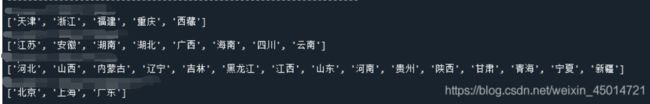
    CityCluster=[[],[],[],[]]      #将城市 按label分成设定的簇，将每个簇的城市输出
    for i in range(len(cityName)):
        CityCluster[label[i]].append(cityName[i])
    for i in range(len(CityCluster)):
        print("Expenses:{}.2f" .format(expenses[i]))
        print(CityCluster[i])

字典和列表的输出

• cityName=[‘北京’,‘上海’,…]是一个包含31个省份名字的列表
• label=[2 0 3 3 3 1 …]含有31个数字代表相应省份所在的蔟。
• label是根据省份消费水平划分的蔟，label里面的0代表第0个蔟，一共有0、1、2、3四个蔟

现在想要把每个蔟里面的省份输出来

CityCluster=[[],[],[],[]]   #四个蔟
for i in range(len(cityName)):
    CityCluster[label[i]].append(cityName[i])
for i in range(len(CityCluster)):
    print(CityCluster[i])

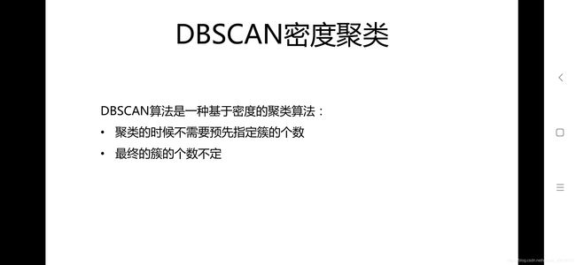
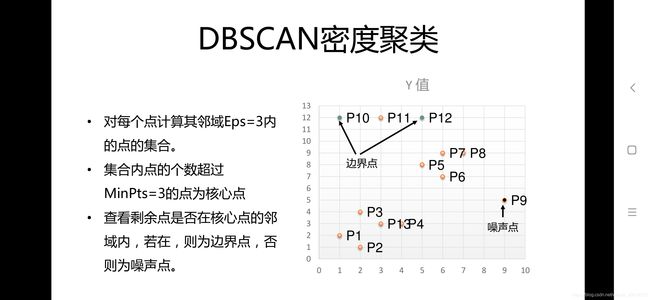
2.无监督学习中的 聚类算法之 Dbscan聚类算法–

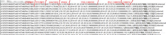
数据请见（电脑F盘）或（腾讯微云文件“Redhur的进阶“）的{python数据—test1}

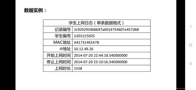
1.根据上网的时间（几点上的网）进行聚类

import numpy as np
import sklearn.cluster as skc
from sklearn import metrics
import matplotlib.pyplot as plt
 
mac2id = dict()
"""
在mac2id这个字典里：
键key是MAC地址
值value是字典里面对应的序号
"""
onlinetimes = []
f = open("F:/python数据/test1.txt",encoding='utf8')
for line in f:
    data = line.split(',')
    mac = data[2] #读取Mac地址
    onlinetime = int(data[6])   #读取上网时长
    starttime =  int(data[4].split(' ')[1].split(':')[0])  #读取开始时间（我们只要年月日时分秒里的“时”）

    mac2id[mac] = len(onlinetimes)  #len(onlinetimes)就是此时对应的onlinetimes里面的元素个数，mac2id的内容见下面
    onlinetimes.append((starttime,onlinetime))#onlinetimes里面的内容见下面

#onlinetimes里面的内容是[(22, 1558), (12, 40261), (22, 1721), (23, 351), (16, 23564),,,]
#mac2id这个字典里面是{'A417314EEA7B': 0, 'F0DEF1C78366': 1, '88539523E88D': 2,,,,'3CDFBD175878': 287, '002427FE3712': 288}

real_X = np.array(onlinetimes).reshape((-1,2)) #参数-1可以自动确定行数

X = real_X[:,0:1] # 截取第一列（也就是“上网时间”），我们是要根据上网的时间进行蔟类

'''
real_X为：
[[    22   1558]
 [    12  40261]
 [    22   1721]
 [    23    351]
 [    16  23564]
 [    23   1162]
 [    22   3540]
 ...
 ]


X为：
[[22]
 [12]
 [22]
 [23]
 [16]
 [23]
 [22]
 ...
 ]
'''

db = skc.DBSCAN(eps=0.01,min_samples=20,metric = 'euclidean').fit(X) #调用Dbscan的的方法进行训练
# eps:两个样本被看作邻居节点的最大距离
# min_sample:簇的样本数
# metrics:距离计算方式（默认欧几里得距离）
 
labels = db.labels_
print("Labels")
print(labels)
ratio = len(labels[labels[:]==-1]) / len(labels) # 判定噪声数据（label被打上-1）数据所占的比例
print("Noise ratio:{:.2f}".format(ratio)) #输出噪声数据所占的比例

n_clusters_ = len(set(labels)) - (1 if -1 in labels else 0)  #减去噪声数据-1占的位置
print("Estimate number of clusters:%d"%n_clusters_)#输出蔟的个数

print("Silhouette Coefficient: %0.3f"% metrics.silhouette_score(X, labels))#输出蔟类效果评价指标（轮廓系数）
#轮廓系数（Silhouette Coefficient）的值是介于 [-1,1] ，越趋近于1代表内聚度和分离度都相对较优
 
for i in range(n_clusters_):
    print("Cluster",i,":")
    print(list(X[labels==i].flatten()))
    # flatten()方法:将numpy对象（如array、mat）折叠成一维数组返回
 
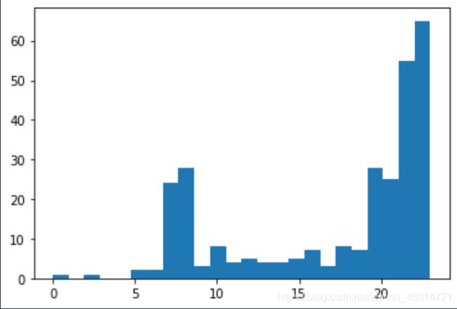
plt.hist(X,24)
plt.show()

相同思想的例题：

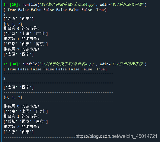
import numpy as np
city=['太原','北京','上海','成都','西安','南京','广州','西宁']
rank=[  2,    0,      0,     1,     1,    1,    0,      2  ] #城市对应的排名
ranks=np.array(rank)
citys=np.array(city)

print(ranks[:]==2)  #[False False False  True  True  True False False]
print('----------------------------------------------------')

num=len( ranks[ranks[:]==2] )   #ranks里面元素等于2的元素的数量（也就是排名第二的城市的数量）
print(num)
print('----------------------------------------------------')

print( citys[ranks[:]==2]  )  #输出排名第二的城市
print('----------------------------------------------------')

print( set(ranks) )
print('----------------------------------------------------')

for i in range( len(set(ranks)) ):
    print('排名第',i,'的城市是：')
    print( citys[ranks[:]==i] )
print('----------------------------------------------------')

2.根据上网的总时长进行聚类

import numpy as np
import sklearn.cluster as skc
from sklearn import metrics

 
mac2id = dict()
"""
key是MAC地址
value是开始上网时间和上网时长
"""
onlinetimes = []
f = open("F:/python数据/test1.txt",encoding='utf8')
for line in f:
    data = line.split(',')
    mac = data[2] #读取Mac地址
    onlinetime = int(data[6])   #读取上网时间
    starttime =  int(data[4].split(' ')[1].split(':')[0])  #读取开始时间（我们只要年月日时分秒里的“时”）

    mac2id[mac] = len(onlinetimes)  #len(onlinetimes)就是此时对应的onlinetimes里面的元素个数，mac2id的内容见下面
    onlinetimes.append((starttime,onlinetime))#onlinetimes里面的内容见下面

#onlinetimes里面的内容是[(22, 1558), (12, 40261), (22, 1721), (23, 351), (16, 23564),,,]
#mac2id这个字典里面是{'A417314EEA7B': 0, 'F0DEF1C78366': 1, '88539523E88D': 2,,,,'3CDFBD175878': 287, '002427FE3712': 288}

#-----------------------------------------以下内容进行了改动-------------------------------------------------------------

real_X = np.array(onlinetimes).reshape((-1,2)) #参数-1可以自动确定行数

X = real_X[:,1:] # 截取第二列（也就是“上网的总时长”）我们这次根据上网的总时长进行蔟类

X=np.log(1+real_X[:,1:])#上网的总时长太大了，都是几千，我们要进行对数化处理
 
db = skc.DBSCAN(eps=0.14,min_samples=10).fit(X) #调用Dbscan的的方法进行训练
# eps:两个样本被看作邻居节点的最大距离
# min_sample:簇的样本数
# metrics:距离计算方式（默认欧几里得距离）
 
labels = db.labels_
print("Labels")
print(labels)
ratio = len(labels[labels[:]==-1]) / len(labels[:]) # 判定噪声数据（label被打上-1）数据所占的比例
print("Noise ratio:{:.2f}".format(ratio)) #输出噪声数据所占的比例
n_clusters_ = len(set(labels)) - (1 if -1 in labels else 0)
print("Estimate number of clusters:%d"%n_clusters_)#输出蔟的个数
print("Silhouette Coefficient: %0.3f"% metrics.silhouette_score(X, labels))#输出蔟类效果评价指标（轮廓系数）
#轮廓系数（Silhouette Coefficient）的值是介于 [-1,1] ，越趋近于1代表内聚度和分离度都相对较优
 
for i in range(n_clusters_):
    print("Cluster",i,":")
    count=len(X[labels==i])
    mean=np.mean(real_X[labels==i][:,1])
    std=np.std(real_X[labels==i][:,1])
    print('\t number of sample:',count)
    print('\t mean of sample:',format(mean,'.1f'))
    print('\t std of sample:',format(std,'.1f'))
 

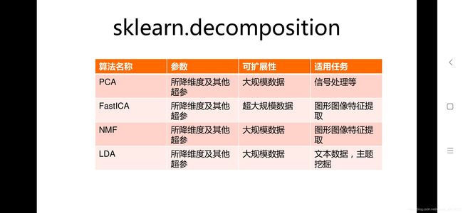
3.无监督学习中的 降维算法之 PCA降维算法–

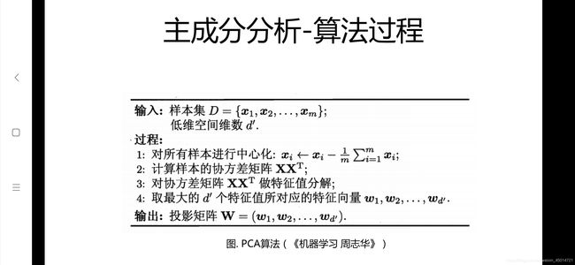
1.直接用numpy进行PCA（不需要看懂）

import numpy as np
n = 2                                         # 取对应特征值最大的n个特征向量
data = np.random.rand(10, 5)                  # （10行5列数据）生成10个样本，每个样本5个特征
mean = np.mean(data, axis=0)                  # 计算原始数据中每一列的均值，axis=0按列取均值
zeroCentred_data = data - mean                # 数据中心化，使每个feature的均值为0
covMat = np.cov(zeroCentred_data, rowvar=False)  # 计算协方差矩阵，rowvar=False表示数据的每一列代表一个feature
featValue, featVec = np.linalg.eig(covMat)    # 计算协方差矩阵的特征值和特征向量
index = np.argsort(featValue)                 # 将特征值按从小到大排序，index是对应原featValue中的下标
n_index = index[-n:]                          # 取最大的n个特征值在原featValue中的下标
n_featVec = featVec[:, n_index]               # 取最大的两维特征值对应的特征向量组成映射矩阵
low_dim_data = np.dot(zeroCentred_data, n_featVec)     # 降维后的数据

2.调用sklearn实现PCA

import numpy as np
from sklearn.decomposition import PCA
data = np.random.rand(10, 5)            # （生成10行5列数据）生成10个样本，每个样本5个特征
pca = PCA(n_components=2)
low_dim_data = pca.fit_transform(data)  # 每个样本降为2维　

3.PCA的参数

sklearn.decomposition.PCA(n_components=None, copy=True, whiten=False)

• n_components: PCA算法中所要保留的主成分个数，也即保留下来的特征个数，如果 n_components = 1，将把原始数据降到一维；
• copy：True 或False，默认为True，即是否需要将原始训练数据复制。
• whiten：True 或False，默认为False，即是否白化，使得每个特征具有相同的方差。

4.PCA对象的属性

• explained_variance_ratio_：返回所保留各个特征的方差百分比，如果n_components没有赋值，则所有特征都会返回一个数值且解释方差之和等于1。
• n_components_：返回所保留的特征个数。

5.PCA常用的方法

• fit(X): 用数据X来训练PCA模型。
• fit_transform(X)：用X来训练PCA模型，同时返回降维后的数据。
• inverse_transform(newData) ：将降维后的数据转换成原始数据，但可能不会完全一样，会有些许差别。
• transform(X)：将数据X转换成降维后的数据，当模型训练好后，对于新输入的数据，也可以用transform方法来降维。

简单的栗子：

import numpy as np
from sklearn.decomposition import PCA
X = np.array([[-1, -1], [-2, -1], [-3, -2], [1, 1], [2, 1], [3, 2]])
pca = PCA(n_components=2)
newX = pca.fit_transform(X)

print(X)
Out[365]: 
[[-1 -1]
 [-2 -1]
 [-3 -2]
 [ 1  1]
 [ 2  1]
 [ 3  2]]
 
print(newX)
Out[366]: 
array([[ 1.38340578,  0.2935787 ],
       [ 2.22189802, -0.25133484],
       [ 3.6053038 ,  0.04224385],
       [-1.38340578, -0.2935787 ],
       [-2.22189802,  0.25133484],
       [-3.6053038 , -0.04224385]])
       
print(pca.explained_variance_ratio_)
[ 0.99244289  0.00755711]

可以发现第一个特征可以99.24%表达整个数据集，因此我们可以降到1维：

pca = PCA(n_components=1)
newX = pca.fit_transform(X)
print(pca.explained_variance_ratio_)
[ 0.99244289]

实例–PCA鸢尾花数据集降维

import matplotlib.pyplot as plt
from sklearn.decomposition import PCA
from sklearn.datasets import load_iris
 
data = load_iris()                 # 以字典形式加载鸢尾花数据集
y = data.target                    # 使用y表示数据集中的标签
X = data.data                      # 使用X表示数据集中的属性数据
pca = PCA(n_components=2)          # 加载PCA算法，设置降维后主成分数目为2
reduced_X = pca.fit_transform(X)   # 对原始数据进行降维，保存在reduced_X中

'''
print(reduced_X)得到：
[[-2.68412563  0.31939725]
 [-2.71414169 -0.17700123]
 [-2.88899057 -0.14494943]
 [-2.74534286 -0.31829898]
 [-2.72871654  0.32675451]
 ...............
 [ 1.90094161  0.11662796]
 [ 1.39018886 -0.28266094]]
'''

red_x, red_y = [], []              # 第一类数据点
blue_x, blue_y = [], []            # 第二类数据点
green_x, green_y = [], []          # 第三类数据点
 
for i in range(len(reduced_X)):    # 按照鸢尾花的类别将降维后的数据点保存在不同的列表中。
    if y[i] == 0:
        red_x.append(reduced_X[i][0])
        red_y.append(reduced_X[i][1])
    elif y[i] == 1:
        blue_x.append(reduced_X[i][0])
        blue_y.append(reduced_X[i][1])
    else:
        green_x.append(reduced_X[i][0])
        green_y.append(reduced_X[i][1])
 
plt.scatter(red_x, red_y, c='r', marker='x')
plt.scatter(blue_x, blue_y, c='b', marker='D')
plt.scatter(green_x, green_y, c='g', marker='.')
plt.show()
#可以看出降维后的数据集仍能够分成三类，并没有改变数据的质量

本实例提取的思想

已知降到2维后的鸢尾花数据集为reduced_X=
[[-2.68412563  0.31939725]
 [-2.71414169 -0.17700123]
 [-2.88899057 -0.14494943]
 [-2.74534286 -0.31829898]
 [-2.72871654  0.32675451]
 ...............
 [ 1.90094161  0.11662796]
 [ 1.39018886 -0.28266094]]

对应的标签为y=
[0 0 0 0 0 0 0 0 0 0 0 0 0 0 0 0 0 0 0 0 0 0 0 0 0 0 0 0 0 0 0 0 0 0 0 0 0
 0 0 0 0 0 0 0 0 0 0 0 0 0 1 1 1 1 1 1 1 1 1 1 1 1 1 1 1 1 1 1 1 1 1 1 1 1
 1 1 1 1 1 1 1 1 1 1 1 1 1 1 1 1 1 1 1 1 1 1 1 1 1 1 2 2 2 2 2 2 2 2 2 2 2
 2 2 2 2 2 2 2 2 2 2 2 2 2 2 2 2 2 2 2 2 2 2 2 2 2 2 2 2 2 2 2 2 2 2 2 2 2
 2 2]

我们要根据标签y里面的数字将reduced_X分开存储到六个列表里

red_x, red_y = [], []              # 第一类数据点
blue_x, blue_y = [], []            # 第二类数据点
green_x, green_y = [], []          # 第三类数据点
 
for i in range(len(reduced_X)):    
    if y[i] == 0:
        red_x.append(reduced_X[i][0])
        red_y.append(reduced_X[i][1])
    elif y[i] == 1:
        blue_x.append(reduced_X[i][0])
        blue_y.append(reduced_X[i][1])
    else:
        green_x.append(reduced_X[i][0])
        green_y.append(reduced_X[i][1])

---

---

以下例题是未搞明白的

---

---

4.无监督学习中的 降维算法之 NMF降维算法–




实例


（以下代码只做了解）

import matplotlib.pyplot as plt
from sklearn import decomposition
#加载PCA算法包
from  sklearn.datasets import fetch_olivetti_faces
#加载人脸数据集
from numpy.random import RandomState
#加载RandomState用于创建随机种子
n_row,n_col = 2,3
#设置图像展示时的排列情况，2行三列
n_components = n_row * n_col
#设置提取的特征的数目
image_shape = (64,64)
#设置人脸数据图片的大小
dataset = fetch_olivetti_faces(shuffle=True,random_state=RandomState(0))
faces = dataset.data#加载数据，并打乱顺序
def plot_gallery(title,images,n_col=n_col,n_row=n_row):
    plt.figure(figsize=(2. * n_col,2.26 * n_row))#创建图片，并指定大小
    plt.suptitle(title,size=16)#设置标题及字号大小
    for i,comp in enumerate(images):
        plt.subplot(n_row,n_col,i+1)#选择画制的子图
        vmax = max(comp.max(),-comp.min())
        plt.imshow(comp.reshape(image_shape),cmap=plt.cm.gray,interpolation='nearest',vmin=-vmax,vmax=vmax)#对数值归一化，并以灰度图形式显示
        plt.xticks(())
        plt.yticks(())#去除子图的坐标轴标签
    plt.subplots_adjust(0.01,0.05,0.99,0.93,0.04,0.)
estimators=[('Eigenfaces - PCA using randomized SVD',decomposition.PCA(n_components=6,whiten=True)),('Non-negative components - NMF',decomposition.NMF(n_components=6,init='nndsvda',tol=5e-3))]
#NMF和PCA实例，将它们放在一个列表中
for name,estimators in estimators:#分别调用PCA和NMF
    estimators.fit(faces)#调用PCA或NMF提取特征
    components_=estimators.components_#获取提取特征
    plot_gallery(name,components_[:n_components])
    #按照固定格式进行排列
plt.show()#可视化

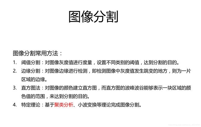
5.基于聚类的"图像分割"实例编写
（未搞明白，未摘抄）

import numpy as np
import PIL.Image as Image #加载PIL包，用于加载创建图片
from sklearn.cluster import  KMeans #加载Kmeans算法

def loadData(filePath):
    data= []
    img=Image.open(filePath)
    m,n =img.size     #获得图片大小（width, height）
    for i in range(m):
        for j in range(n):
            x,y,z =img.getpixel((i,j))   #im.getpixel(x,y)返回给定位置的像素值。
            data.append([x/256.0,y/256.0,z/256.0])#将每个像素点RGB颜色处理到0-1范围内,将颜色值存入data内
    return np.mat(data),m,n #以矩阵的形式返回data，以及图片大小

imgData,row,col =loadData('bull.png') #调用函数，获取数据
km=KMeans(n_clusters=3) #聚类获得每个像素所属的类别
label =km.fit_predict(imgData)
label=label.reshape([row,col])

pic_new = Image.new("L",(row,col))#创建一张新的灰度图以保存聚类后的结果

for i in range(row):
    for j in range(col):
        pic_new.putpixel((i,j),int(256/(label[i][j]+1))) #im.putpixel((x,y),(r,g,b)) 在指定位置(x,y)处画一像素

pic_new.save("result-bull-4.jpg","JPEG") #以JPEG格式保存图像