认识小波——MATLAB中国的讲座(笔记)
第一部分:什么是小波
https://www.bilibili.com/video/BV1xu411R7yK
现实世界中的数据或信号经常表现出缓慢变化的趋势或者有瞬变的振荡
Real world data or signals frequently exhibit slowly changing trends or oscillations punctuated with transients
图像的平滑区域会被边缘突变或对比度突变打断,无论在感知上还是在提供的信息方面,这些突变通常是数据中最令人感兴趣的部分
傅里叶变换是数据分析的强大工具,但是它不能有效地表示突变,这是因为傅里叶变换将数据表示为正弦波之和。而正弦波在时间或空间上都不是局部化的。正弦波永远在振荡。

因此,为了准确地分析具有突变的信号和图像,我们需要使用一类在时间和频率上具有良好局部化特性的新函数,这就引出了小波的主题。
小波是一种具有零均值的快速衰减的波浪状振荡
A wavelet is a rapidly decaying, wave-like oscillation that has zero mean
与扩展到无穷远的正弦波不同,小波存在的时间有限
Unlike sinusoids, which extend to infinity, a wavelet exists for a finite duration
小波有不同的大小和形状
Wavelets come in different sizes and shapes

小波分析具有广泛的适用性,这是小波分析的一个重要优点
The availability of a wide range of wavelets is a key strength of wavelet analysis
要选择合适的小波,您需要考虑它的应用领域,我们将在随后的课程中详细地说明这一点
To choose the right wavelet, you’ll need to consider the application you’ll use it for, We will discuss this in more detail in a subsequent session
现在,让我们关注两个重要的小波变换概念,缩放和平移
For now, let’s focus on two important wavelet transform concepts, scaling and shifting.
缩放 scaling
假设你有一个信号PSI(t),
缩放是指在时间上拉伸或收缩信号的过程
Scaling refers to the process of stretching or shrinking the signal in time

S是尺度因子,它是正值,对应于信号在时间上的尺度。尺度因子与频率成反比。
S is the scaling factor,which is a positive value and corresponds to how much a signal is scaled。The scale factor is inversely proportional to frequency。
例如,将正弦波缩放2会导致其原始频率降低一或一个倍频程
scaling a sine wave by 2 results in reducing its original frequency by half or by an octave

对于小波,尺度和频率之间存在一个比例常数的倒数关系。这个比例常数称为小波的“中心频率”
there is a reciprocal relationship between scale and frequency with a constant of proportionality。This constant of proportionality is called the"center frequency"of the wa velet

与正弦波不同,小波在频域中具有带通特性
unlike the sinewavethe wavelet has a band pass characteristic in the frequency domain
从数学上讲,等效频率是使用[屏幕上]这个等式定义的
Mathematically,the equivalent frequency is defined using this equation[on screen]
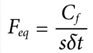
其中Cf是小波的中心频率,s是小波尺度,At是采样间隔
where Cf is center frequency of the wavelet,s is the wavelet scale,and delta t is the sampling interval
因此,当您将小波缩放2倍时,将导致等效频率降低一个倍频程
Therefore when you scale a wavelet by a factor of 2,it results in reducing the equivalent frequency by an octave
此处显示的是中心频率为0.71Hz的sym4小波,如何对应于相同频率的正弦波
here is how a sym4 wavelet with center frequency 0.71 Hz corresponds to a sine wave of same frequency
较大的尺度因子会生成拉伸的小波,对应于较低的频率
A larger scale factor results in a stretched wavelet which corresponds to a lower frequency
较小的尺度因子会生成收缩的小波,对应于高频
A smaller scale factor results in a shrunken wavelet which corresponds to a high frequency

拉伸小波有助于捕获信号中缓慢发生的变化,而压缩小波有助于捕获突变
A stretched wavelet helps in capturing the slowly varying changes in a signal,while a compressed wavelet helps in capturing abrupt changes
如前所述,您可以构建与等效频率成反比的不同尺度
You can construct diferent scales that inversely correspond the equivalent frequencies
移位 shifting
移动小波意味着沿信号长度延迟或提前小波的开始
Shifting a wavelet simply means delaying or advancing the onset of the wavelet along the length of the signal
用此符号表示的移位小波[在屏幕上],表示小波已移位并以k为中心
A shifted wavelet represented using this notation[on screen],means that the wavelet is shifted and centered at k

我们需要移动小波,使其与我们在信号中寻找的特征对齐
We need to shit the wavelet to align with the feature we are looking for in a signal
小波分析中的两种主要变换是连续小波变换和离散小波变换,这些变换根据小波的缩放和移位方式而有所不同
The two major transforms in wavelet analysis are Continuous and Discrete Wavelet Transforms。These transforms differ based on how the wavelets are scaled and shifted
第二部分:小波变换的类型
https://www.bilibili.com/video/BV14m4y1d7kp
连续小波分析的主要应用是时频分析和时间局部化频率分量的过滤
Key applications of the continuous wavelet analysis are time frequency analysis,and filtering of time localized frequency components
离散小波分析的关键应用是 信号和图像的去噪和压缩
The key application for Discrete Wavelet Analysis are denoising and compression of signals and images
这两种变换的不同之处在于它们离散化尺度和平移参数的方式,我们将讨论这些技术在1-D场景中的应用
these two transforms differ based on how they discretize the scale and the translation parameters。We will discuss these techniques as they apply in the 1-D scenario
连续小波变换 Continuous Wavelet Transform
您可以使用此转换来获得信号的同步时频分析
You can use this transform to obtain a simultaneous time frequency analysis of a signal
解析小波最适合于时频分析,因为这些小波没有负的频率分量
Analytic wavelets are best suited for time frequency analysis as these wavelets do not have negative frequency components。
此列表包括一些适用于连续小波分析的分析小波
This list includes some analytic wavelets that are suitable for continuous wavelet analysis
·Morse Wavelets
·Bump Wavelet
·Analytic Morlet Wavelet

CWT的输出是系数,这些系数将用作尺度或者频率和时间的函数
The output of CWT are coefficients which are a function of scale or frequency and time
现在,让我们来讨论构造不同小波尺度的过程
Let’s now discuss the process of constructing different wavelet scales
回想一下我们之前的视频,当您将小波缩放2倍时,它会将等效频率降低一个倍频程
Recall from our previous video that when you scale a wavelet by a factor of 2,it results in reducing the equivalent frequency by an octave
凭借 CWT,您可以更灵活地在每个倍频程内以中间尺度分析信号
With the CWT you have the added flexibility to analyze the signal at intermediary scales within each octave
这允许进行精细尺度分析,此参数称为每倍频程的尺度数(Nv)
This allows for fine scale analysis,This parameter is referred as the number of scales per octave(Nv)
每倍频程的长度数越大,尺度离散化越精细
The higher the number of scales per octave,the finer the scale discretization
此参数的典型值为10、12、16和32
Typical values for this parameter are 10,12,16,and 32
尺度与信号的采样间隔相乘,可获得物理意义
The scales are multiplied with the sampling interval of the signal to obtain a physical significance
现在,每个缩放的小波沿信号的整个长度进行时间偏移并与原始信号进行比较。
Now,each scaled wavelet is shifted in time along the entire length of the signal and compared with the original signal
您可以对所有尺度重复此过程,从而生成作为小波尺度和移位参数函数的系数
You can repeat this process for all the scales resulting in coefficients that are a function of the wavelet’s scale and shift parameter
客观来看,一个包含1,000个样本的信号用20个尺度分析会产生20,000个系数a signal with
To put it in perspective 1000 samples analyzed with 20 scales results in 20,000 coefficients.
这样,您可以使用连续小波变换更好地表征信号中的振荡行为
In this way,you can better characterize oscillatory behavior in signals with the Continuous wavelet transform
离散小波变换(DWT)
离散小波变换(DWT)是对信号和图像进行去噪和压缩的理想选择,因为它有助于用较少的系数表示许多自然发生的信号和图像.这使得表示更为稀疏
The discrete wavelet transform or DWT is ideal for denoising and compressing signals and images as it helps represent many naturally occurring signals and images with fewer coefficients. This enables a sparser representation
DWT中的基本尺度设置为2,通过将此基本尺度提升为以这种方式表示的整数值,您可以获得不同的尺度
The base scale in DWT is set to 2,You can obtain different scales by raising this base scale to integer values represented in this way
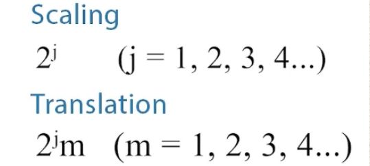
平移发生在该等式中表示的整数倍处,这个过程通常被称为二元缩放和移位
The translation occurs at integer multiples represented in this equation,This process is often referred to as a dyadic scaling and shifting
这种采样消除了系数的冗余
This kind of sampling eliminates redundancy in coefficients
变换的输出会生成与输入信号长度相同数量的系数。因此,它需要的内存更少
The output of the transform yields the same number of coefficients as the length of the input signal。Therefore,it requires less memory
离散小波变换过程相当于将信号与离散多速率滤波器组进行比较
The discrete wavelet transform process is equivalent to comparing a signal with discrete multirate filter banks
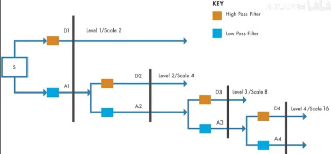
从概念上讲,它是这样工作的,假定有一个信号-S-,该信号首先用特殊的低通和高通滤波器进行滤波,以产生低通和高通子带。我们可以-将其称为A1和D1,根据奈奎斯特准则过滤后,一半的样本被丢弃,这些滤波器通常具有少量系数,并能产生良好的计算性能
Conceptually,here is how it works,Given a signal-S-,the signal is first filtered with special lowpass and high pass filter to yield lowpass and highpass sub-bands。We can-refer to these as Al and D1,Half of the samples are discarded after filtering as per the Nyquist criterion,The filters typically have a small number of coefficients,and result in good computational performance
这些滤波器还能够重建子带,同时消除由于下采样而发生的任何混叠。
These filters also have the ability to reconstruct the sub bands,while cancelling any aliasing that occurs due to downsampling
对于下一级分解,低通子带(A1)使用相同的技术进行迭代滤波,产生更窄的子带-A2和D2,依此类推
For the next level of decomposition,the lowpass subband(A1)is iteratively filtered by the same technique to yield narrower subbands-A2 and D2 and so on.
每个子带中系数的长度是前一级中系数数量的一半
The length of the coefficients in each sub band is half of the number of coefficients in the preceding stage
使用此技术,您可以捕获具有几个幅值较大的DWT系数的重要信号,而信号中的噪声会生成较小的DWT系数
With this technique you can capture the signal of interest with a few large magnitude DWT coefficients,while the noise in the signal results in smaller DWT coefficients
通过这种方式,DWT有助于分析不同分辨率下逐渐变窄的子带上的信号,它还有助于去噪和压缩信号
This way,the DWT helps analyze signals at progressively narrower subbands at different resolutions,It also helps denoise and compress signals。
第三部分:离散小波变换的示例应用
https://www.bilibili.com/video/BV1wP4y1A7n3
使用小波对信号进行去噪,同时保留其清晰的特征。 该视频概述了使用 MATLAB® 通过离散小波变换对信号进行去噪所涉及的步骤。
了解这种去噪技术与其他去噪技术的比较。 使用小波分析并合成信号和图像,了解并获取Wavelet
Toolbox工具箱试用:https://bit.ly/3Heyacc 获取视频中代码下载:https://bit.ly/3EOtcSd
----------------------------------------------------------------------------- © 2021 The MathWorks, Inc. MATLAB and Simulink are registered
trademarks of The MathWorks, Inc. See www.mathworks.com/trademarks for
a list of additional trademarks. Other product or brand names maybe
trademarks or registered trademarks of their respective holders
让我们加载一个信号并在MATLAB中绘制它,这里有两个信号,第一个是原始信号,第二个是添加了一些噪声的原始信号
Let us load a signal and plot it in MATLAB。There are two signals here,The first is the original signal and the second one is the original signal with some noise added to it
我们的目标是使用离散小波变换对噪声信号进行去噪
Our goal here is to denoise the noisy signal using the discrete wavelet transform
小波去噪的步骤概述
以下是小波去噪的步骤概述
Here is an overview of the steps involved in wavelet denoising
1.第一步是获得近似系数和细节系数,通过执行多级小波分解可做到这一点
1.Your first step is to obtain the approximation and the detail coefficients,Do this by performing a multilevel wavelet decomposition
我们之前讲过,离散小波变换会将信号分成低通子带(也称为“近似级”),和高通子带(也称为“细节级”)
Recall that the discrete wavelet transform splits up a signal into a low pass subband(also called the“approximation level")and high pass subband(also called the“detail level")
您可以在多个级别或尺度上分解近似子带以进行精细尺度分析
You can decompose the approximation subband at multiple levels or scales for a fine scale analysis
2.第二步是分析细节并确定合适的阈值技术
2.The second step is to analyze the details and identify a suitable thresholding technique
3.第三步是对细节系数进行阈值处理并重构信号
3.The third step is to threshold the detail coefficients and reconstruct the signal
wavedec函数
让我们首先使用函数wavedec执行多级小波分解
Let us first perform a multilevel wavelet decomposition using the function wavedec
我们将使用sym6小波并将噪声信号分解为五个级别
We will use a sym6 wavelet and decompose the noisy signal down to five levels
dwtmode('per','nodisplay');
wname = 'sym6';
level = 5;
[C, L] = wavedec(f,level,wname);
该函数输出第5级近似系数,以及从1级到5级的细节系数
The function outputs the fifth level approximation coefficients along with the detail coefficients from levels one through five
第1级细节系数会捕捉信号的高频,大多数高频成分都包含信号中存在的噪声,然而,高频部分是由信号的突变构成的。有时,这些突变具有意义,您可能希望在去除噪音的同时保留这些信息
The first-level detail coefficients capture the high frequencies of the signal,Most of the high frequency content comprises the noise present in the signal。However,part of the high frequency is made up of abrupt changes in the signal。There are times when these abrupt changes carry meaning,and you would want to retain this information while removing the noise。
detcoef函数
让我们仔细看看细节子带,要提取系数,您可以使用detcoef函数并绘制每个级别的系数。
Let us take a closer look at the details subband,To extract the coefficients,you can use the detcoef function and plot the coefficients for each level。
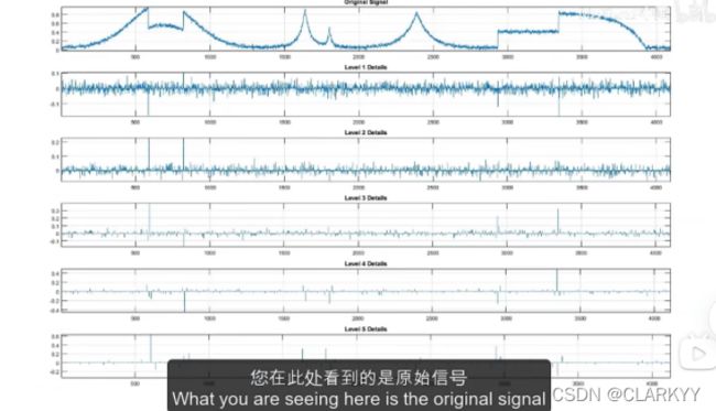
我将使用一个辅助函数来提取和绘制系数,您在此处看到的是原始信号,以及为1到5级绘制的详细信息。
I am using a helper function to extract and plot the coefficients,What you are seeing here is the original signal along with the details plotted for levels one through five。
请注意,随着尺度或级别的增加,活动急剧减少。因此,我们将专注于第1级细节,暂时忽略其余部分。我们的目标是在消除噪音的同时保留这些剧变。
Notice that the activity reduces drastically as the scale or level increases。So,we will focus on the level one details and ignore the rest for now。Our aim here is to retain these sharp changes while getting rid of the noise。
一种方法是通过阈值来缩放细节系数,
One way to do this is by scaling the detail coefficients by a threshold,
Thresholding Techniques
The universal threshold
SureShrink or the 'rigrsure’method
The Heursure method
The minimax method
MATLAB中有四种主要技术可帮助您计算用于去噪目的的阈值
There are four main techniques available in MATLAB to help you compute a threshold for the purpose of denoising,
通用阈值是最容易计算的,并使用此公式计算
The universal threshold is the simplest to compute and is computed using this formula
手动计算其他三种去噪技术的阈值并不那么简单.您可使用MATLAB实现这一点,这样您就可以专注于阈值的使用,而不必担心如何计算阈值
Manually computing the threshold for the other three denoising techniques is not as straightforward.Instead,you can use MATLAB for this so that you can focus on using the threshold value without worrying about how it is computed.
有两种应用阈值的方法,软阈值和硬阈值.在这两种情况下,幅值小于阈值的系数都设置为0
There are two ways of applying the threshold, soft thresholding and hard thresholding.In both cases the coefficients with a magnitude less than the threshold are set to zero.
这两种闽值操作的区别在于它们处理幅值大于阈值的系数的方式
The difference between these two thresholding operations lies in how they deal with coefficients that are greater in magnitude than the threshold.
在应用软阈值的情况下,通过从系数值中减去阈值,将幅值大于阈值的系数收缩为0(?趋向0)。而在硬阈值处理中,幅值大于阈值的系数保持不变
In the case of soft thresholding,the coefficients greater in magnitude than the threshold are shrunk towards zero by subtracting the threshold value from the coefficient value;whereas in hard thresholding,the coefficients greater in magnitude than the threshold are left unchanged
回到我们的示例,让我们使用SureShrink 和软阈值技术对噪声信号进行降噪
Coming back to our example,let us denoise our noisy signal using Sure Shrink with the soft thresholding technique
对系数进行阈值处理,和从新系数重构信号的整个过程可以使用单个函数完成,如下所示
The entire process of thresholding the coefficients,and reconstructing the signal from the new coefficients can be done using a single function,as shown here
fd = wden(f,'rigrsure','s','sln',level,wname);
第一个参数f是噪声信号。第二个参数指定阈值技术。在这种情况下是SureShrink。s表示软阈值处理。参数sln表示使用基于第1级系数的单个噪声估计值进行阈值重缩放。level 表示小波分解级别。最后一个参数指定小波,在本例中为sym6
The first parameter,f,is the noisy signal。The second parameter specifies the thresholding technique。In this case is Sure Shrink。s denotes soft thresholding。and the parameter sln indicates threshold rescaling using a single estimate of noise based on first-level。level indicates the wavelet decomposition level。and the last parameter specifies the wavelet which is sym6 in this case。
函数wden 对输入信号执行多级分解,计算阈值并将其应用于细节系数,使用新的细节系数重构信号,并将其作为输出提供
The function wden performs a multilevel decomposition of the input signal,computes and applies the threshold to the detail coefficients, reconstructs the signal with the new detail coefficients and provides it as an output。
现在让我们使用plot命令,将噪声信号与去噪信号(上一步的输出)进行比较,显然去噪版本的噪声更少
Let us now use the plot command to compare the noisy signal with the denoised signal which was the output of the previous step.Clearly,the denoised version has less noise
您还可以将我们之前讨论的去噪技术的性能与其他去噪技术(例如Savitzky-Golay 滤波或移动平均技术)进行比较,可以看到小波去噪方法优于其他去噪技术
You can also compare the performance of the denoising technique we discussed earlier with other denoising techniques such as Savitzky-Golay filtering or the moving average technique,You can see that the wavelet denoising method outperforms other denoising techniques.
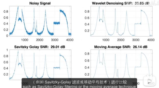
因此,使用小波技术对信号去噪的好处是显而易见的
In this way,the benefits of using wavelet techniques to denoise a signal are clear.
第四部分:连续小波变换的示例应用
https://www.bilibili.com/video/BV1YL4y1g76Q
我将演示如何使用连续小波变换对信号进行理想的时频分析
I will illustrate how to obtain a good time-frequency analysis of a signal using the Continuous Wavelet Transform
首先,让我们在MATLAB中加载地震信号,该信号以1Hz的频率采样,持续51分钟,您可以使用plot命令查看信号
To begin,let us load an earthquake signal in MATLAB,This signal is sampled at 1 Hz for a duration of 51 minutes。You can view the signal using the plot command。
通过观察信号的时域表示,我们会看到两个不同的区域。第一次地震活动发生在30分钟左右,持续很短的时间,第二次地震活动发生在34分钟左右,时间相对较长。
Looking at the time domain representation of the signal,we see two distinct regions。The first seismic activity occurs around the 30 minute mark,This lasts for a very short duration。The second seismic activity occurs sometime around 34 minutes and is relatively longer。

您可以看到,仅通过查看时域表示很难将噪声与地震信号分离。许多自然发生的信号具有相似的特征,它们由缓慢变化的成分组成,中间穿插着剧变并且经常被噪音所掩盖。
You can see,how it is difficult to separate the noise from the seismic signals just by looking at the time-domain representation。Many naturally occurring signals have similar characteristics,They are composed of slowly varying components interspersed with abrupt changes and are often buried in noise。
小波在分析这类信号时非常有用,我们将在稍后做介绍
Wavelets are very useful in analyzing these kinds of signals。We will see how a bit later。
但首先,让我们看看当使用短时傅立叶变换生成时频显示时会发生什么。我们将信号和采样频率作为输入参数传递给函数谱图。
But first,let us see what happens when we use the short time Fourier transform to produce a time-frequency visualization。We pass in the signal and the sampling frequency as input arguments to the function spectrogram。

您可以看到我们刚刚看到的两个地震活动实例现在无法区分
you can see that the two instances of seismic activity we just saw are now indistinguishable
我们所看到的只是一个信号,其频率分布在0.05Hz左右,但没有很好地局部化。
All we see is a signal,whose frequency is spread around 0.05 Hz but is not very well localized
让我们看看当我们尝试通过减少频谱图中使用的窗口大小来局部化事件时会发生什么
Let us see what happens when we try to localize the events by reducing the window size used in the spectrogram
spectrogram(kobe,128,[],[],Fs,'yaxis');
通过减小窗口的大小,我们在30和33分钟左右看到了一些亮点,但是这两个事件并没有很好地分开。事件的频率和时间的不确定性仍然很高。减小窗口大小并不是很有帮助
By reducing the size of the window,we see some bright spots around 30 and 33 mins
but the two events are not well separated。The frequency and time uncertainty of the events is still very high,Reducing the window size was not very helpful。
CWT
我们需要以某种方式局部化这两个事件的频率信息,现在让我们再次进行分析——这次使用小波。我们将使用MATLAB中的CWT函数,来计算连续小波变换。这将有助于获得地震数据的时频联合分析
We need to somehow localize the frequency information of these two events,Now let us repeat the analysis-this time using wavelets。We will use the CWT function in MATLAB to compute the Continuous Wavelet Transform。This will help obtain a joint time frequency analysis of the earthquake data
Continuous Wavelet Transform
Morse Wavelets
Analytical Morlet
Bump Wavelet
CWT函数支持这些关键的解析小波。如果不指定要使用哪个小波,CWT会默认使用莫尔斯小波。当未指定输出参数时,CWT函数会生成输入信号的时频联合显示
The CWT function supports these analytic key wavelets。If you don’t specify which wavelet you want to use,the CWT uses morse wavelets by default。When no output parameters are specified the function,CWT produces a joint time-frequency visualization of the input signal

用于分析的最小和最大尺度,由CWT函数根据小波的能量传播自动确定。
The minimum and maximum scales for analysis are determined automatically by the CWT function based on the wavelet’s energy spread
函数返回的小波系数的幅值用颜色编码,自色虚线表示影响范围。在此区域内,小波系数估计是可靠的。
The magnitude of the wavelet coefficients returned by the function are color coded。The white dashed lines denote the cone of influence。Within this region the wavelet coefficient estimates are reliable。
从图中,可以看出发生地震的两个区域。第一次地震活动与第二次明显分开了。这两个事件似乎在时间和频率上都得到了很好的局部化
Looking at the plot,we can see the two regions produced by the earthquake。The first seismic activity is clearly separated from the second。Both these events seem to be well localized in time and frequency。
对于更丰富的时频分析,您可以选择改变要用于执行分析的小波尺度,您可以通过使用不同的参数来实现这一点
For a richer time-frequency analysis,you can choose to vary the wavelet scales over which you want to carry out the analysis,You can do this by using different parameters
No = 10;
Nv = 32;

cwt(kobe,Fs, 'NumOctaves' ,No,'VoicesPerOctave',Nv);
在本例中,我们将倍频带数量设置为10,每个倍频带的声音数量设置为32。该函数返回小波系数和等效频率作为输出
For this example,we will set the number of octaves to 10,and the number of voices per octave to 32。The function returns the wavelet coefficients and the equivalent frequencies as outputs。
我们可以使用surface命令绘制系数a作为时间和频率图的函数
We can plot the coefficientsra as function of time and frequency plot,using the surface command Hz

从这幅图上看,很明显,地震事件的频率范围为0.03Hz至0.06
Looking at this plot,it is clear that the frequency of the seismic event ranges from 0.03 Hz to 0.06 Hz
ICWT
[WT, F] = cwt(kobe,Fs);
xrec = icwt(WT, F, [0.03 0.06],'SignalMean',mean(kobe));
我们还可以使用函数icwt从小波系数重构此地震事件的时域表示,我们传人了小波系数WF和频率向量F,这是CWT函数的输出
We can also reconstruct the time-domain representation of this seismic event from the wavelet coefficients using the function icwt。We pass in the wavelet coefficients and the frequency vector which is the output of the CWT function
我们还传递了要提取的信号的频率范围,在本例中,我们输入的是0.03到0.06。输出是重要地震信号的时域表示
We also pass the frequency range of the signal that we want to extract,In this case,we’re inputting 0.03 to 0.06。The output is a time-domain representation of the seismic signal of interest

如上所示,您可以使用小波进行时频联合分析
This way,you can use wavelets for performing joint time-frequency analysis
第五部分:在机器学习和深度学习中使用小波散射
https://www.bilibili.com/video/BV1y44y1T7n1
在本视频中,我们将讨论小波散射变换,以及如何将其用作自动化鲁棒特征提取器进行分类,我们将介绍小波散射技术对信号的处理,但同样的技术也可以应用于图像
In this video,we will discuss wavelet scattering transform and how it can be used as an automatic robust feature extractor for classification.We will cover the working of the wavelet scattering technique for signals,but the same technique can also be applied to images
深度卷积网络
小波散射最好在深度卷积网络(深度CNN)的上下文中理解,你们中有些人可能已经熟悉了深度卷积网络
Wavelet scattering is best understood in the context of deep convolutional networks or deep CNNs which some of you may already be familiar with
在高层次上,深度卷积网络会过滤数据,应用一些非线性,并对输出进行池化或平均,重复这些步骤可形成层,
At a high level,deep convolutional networks filter the data apply some nonlinearity and pool or average the output,These steps are repeated to form the layers,
深度CNN面临着一些挑战
There are a few challenges with deep CNNs
1.这些模型通常需要大数据集和大量计算资源来进行训练和评估
These models typically require large datasets and significant computing resources for training and evaluation
2.通常,您必须为网络选择多个设置,这些设置不会对性能造成独立的影响
you must choose many settings for your networks which do not independently affect performance.
3.理解和解释提取的特征可能很困难
It can be difficult to understand and interpret the features that are extracted
小波散射 wavelet scattering
现在您已经了解了这些背景,接下来,让我们看看小波散射如何解决这些挑战
Now that you have this background,let’s see how wavelet scattering addresses these challenges
最初促使人们使用小波散射网络的,是一组已知的滤波器,因为经过充分训练的网络中的滤波器通常类似于类小波滤波器,主要区别在于卷积神经网络情况下的滤波器权重是习得的,而小波散射网络情况下的滤波器权重是固定的
The motivation behind using wavelet scattering networks is to start with a set of known filters since the filters in fully trained networks often resemble wavelet-like filters,The main difference is that the filter weights are learned in the case of convolutional neural networks,while the filter weights are fixed in the case of wavelet scattering networks
现在,让我们深入了解网络的细节
Now,let’s dive into the details of the network
首先使用小波低通滤波器对输入信号进行平均,这是第0层散射功能,通过平均操作,您会丢失信号中的高频细节。
|An input signal is first averaged using wavelet lowpass filters,This is the Layer-0 scattering feature。With the averaging operation,you lose high-frequency detail in the signal
对信号执行连续小波变换可生成一组尺度图系数,这允许在后续层中捕获在第一步中丢失的细节。将非线性算子(在本例中为模数)应用于尺度图系数,然后使用小波低通滤波器对输出进行滤波,从而生成一组第一层散射系数
The details lost in the first step are captured at the subsequent layer by performing a continuous wavelet transform of the signal to yield a set of scalogram coefficients.A nonlinear operator(in this case a modulus)is applied on the scalogram coefficients,and then the output is filtered with the wavelet lowpass filter yielding a set of Layer-1 scattering coefficients
重复相同的过程以获得第2层散射系数,也就是说,上一层尺度图系数的输出,将成为下一层操作的输入,然后我们应用相同的模运算符,并利用小波低通函数对输出进行滤波,得到第2层散射系数
The same process is repeated to obtain the Layer-2 scattering coefficients,meaning,the output of the scalogram coefficients in the previous layer,becomes the input to the operations in the next layer,Then we apply the same modulus operator,and filter the output with the wavelet lowpass function to yield the Layer-2 scattering coefficients。

散射网络可以包含三层以上,但实际上每次迭代都会耗散能量,因此对于大多数应用来说,三层就足够了。通常会对系数进行下采样以降低网络的计算复杂度,这些系数统称为散射特征。您还可以可视化和解释这些特征。
but in practice the energy dissipates with every iteration,so three layers are enough for most applications。The coefficients are typically downsampledto reduce the computational complexity of the network。These coefficients are collectively referred to as the scattering features,You can have more than three layers in the scattering network。You can also visualize and interpret these features
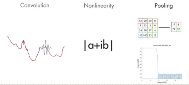
小波散射网络被称为深度网络,因为它会执行构成深度网络的三个主要任务:卷积、非线性和池化
A wavelet scattering network is referred to as a deep network,because it performs the three main tasks that make a deep network:Convolution,Nonlinearity,and Pooling
在这种情况下,卷积由小波执行,模运算符用作非线性化,并且小波低通滤波器的滤波类似于池化。
In this case,convolution is performed by wavelets,the modulus operator serves as the nonlinearity,and filtering with wavelet lowpass filters is analogous to pooling
通过这种方式,您可以使用从小波散射网络获得的特征,并构建可以对数据进行分类的模型
This way,you can use the features obtained from the wavelet scattering network and build models that can classify your data。
有关更多信息和示例,请参阅 Wavelet Toolbox的文档部分
For more information and examples,please refer to the documentation section of Wavelet Toolbox
mathworks.com/wavelet-scattering