TwoSampleMR-R教程 两样本孟德尔随机化（原来真的就是这么简单……）

1. 工具变量

install.packages("remotes")
remotes::install_github("MRCIEU/TwoSampleMR")##To update the package just run the command again
install.packages("readxl")

读取本地文件

1. 方法1：先改变量名，然后format_data()读取自己整理好的工具变量文件，命名如下图。注意，命名区分大小写，不正确则无法读取
   

##name:SNP	beta	se	effect_allele	eaf	exposure	chr	position	gene	pval	samplesize	mr_keep
HcyIV <- as.data.frame(read_excel("IV_Hcy.xlsx"))
library(TwoSampleMR)
Hcy_exp_dat <- format_data(HcyIV, type="exposure")

2. 方法2：直接用read_exposure_data()读，然后code改。尽可能提供多的信息，方便后期画图

HcyIV.2 <- read_exposure_data(
  filename = "IV_Hcy2.csv",
  sep = ",",
  snp_col = "SNP",
  beta_col = "beta",
  se_col = "se",
  effect_allele_col = "effect_allele",
  #other_allele_col = "a2",
  eaf_col = "eaf",
  pval_col = "pval",
  #units_col = "Units",
  #gene_col = "Gene",
  samplesize_col = "samplesize"
)

3. 最后改好自己的暴露名

Hcy_exp_dat$exposure <- "Homocysteine"

工具变量必须为独立变量。根据参考文献选择ref人群和r2

## Clumping via IEU GWAS database
Hcy_exp_dat_clumped <- clump_data(Hcy_exp_dat, clump_r2 = 0.2, pop="EUR")
# default using EUR population from 1000 Genomes project
## Read reference for suitable r2

2. 结局变量

选好工具变量之后，就要将工具变量从结局的GWAS中提取出来。
可以像上面一样从本地读取，也可以从R包里提。下面展示从R包提取的方法。

从数据库获取结局相关的GWAS

## Get GWAS data from the IEU GWAS database that rooted in the package 
ao <- available_outcomes()
#> API: public: http://gwas-api.mrcieu.ac.uk/
ao_outcome <- ao[grepl("stroke", ao$trait), ]
View(ao_outcome)

一个trait很多实验，一个实验一个id；实验来自不同人群和biobank，选择最新的样本量最大的高质量的研究（看year and author）、选择相应研究的id。
选择Ischemic stroke的id是

ieu-a-1108

也可以直接到网站查找，可以顺便查看id Batch的细节。

https://gwas.mrcieu.ac.uk/

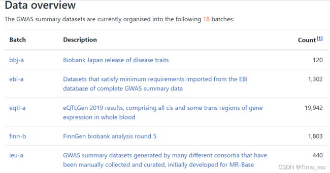
但更建议手动查找，因为网站不全！

从结局GWAS提取工具变量

IS_out_dat <- extract_outcome_data(
  snps = Hcy_exp_dat_clumped$SNP, # use data after clumping
  outcomes = 'ieu-a-1108',
  proxies = TRUE, #default
  rsq=0.8, #default; min is 0.6
  palindromes = 1, #Allow palindromic SNPs? Default is 1 (yes)
  maf_threshold = 0.3 #If palindromes allowed then what is the maximum minor allele frequency of palindromes allowed? Default is 0.3.
)

软件会自动根据LD选取proxy，default R2=0.8

Extracting data for 18 SNP(s) from 1 GWAS(s)
Finding proxies for 1 SNPs in outcome ieu-a-1108
Extracting data for 1 SNP(s) from 1 GWAS(s)

注意网上extract默认允许palidromes。Palidrome是啥？

A palindromic SNP (also known as an ‘ambiguous’ SNP) is a SNP in which the possible alleles for that SNP pair with each other in the double helix structure

Palidrome就是“回文序列”，简单来说就是，A/T、C/G这样的结构。如图所示，A1=A，A2=T，无法根据A1和A2来判断暴露和结局的两个SNP是否方向一致（因为A对应就是T，T对应就是A）。此时就需要根据allele frequency来判断。如下图，暴露的eaf=0.11，如果结局也是和暴露一个方向，其eaf也应该在0.11左右（默认可接受差距=0.3）；但是其eaf=0.91，太大了。所以我们推断，结局allele的方向和暴露的相反，所以其效应effect应该反过来= - (-0.05)=0.05

注意：如结局summary是本地文件，建议根据IV，merge得到结局summary，然后手动检查和判断回文结构。因为下一步harmonize是没有再allow palindromic的选项了。

harmonising的时候默认所有序列都是顺读的（presented on the forward strand）。

3. 数据预处理

对数据进行预处理，使其效应等位与效应量保持统一，就是调整exp和out上位点的方向和beta，使其统一。

## To harmonise the
dat <- harmonise_data(
  exposure_dat = Hcy_exp_dat, 
  outcome_dat = IS_out_dat)

4. MR和敏感性分析等

## MR
res <- mr(dat)

## Heterogeneity statistics
mr_heterogeneity(dat)

# pleiotropy test
mr_pleiotropy_test(dat)


# leave-one-out analysis
res_loo <- mr_leaveoneout(dat)

默认五种方法：MR Egger、Weighted median、Inverse variance weighted、Simple mode和Weighted mode
用mr_method_list() 查看当前支持的其他统计方法。
在mr函数中添加想要使用的方法

mr(dat, method_list=c("mr_egger_regression", "mr_ivw"))

5. 可视化

# scatter plot
p1 <-mr_scatter_plot(res, dat)
length(p1) # to see how many plots are there
p1[[1]]

# forest plot
res_single <- mr_singlesnp(dat)#,all_method=c("mr_ivw", "mr_two_sample_ml")) to specify method used
p2 <- mr_forest_plot(res_single) 
p2[[1]]

## funnel plot for all
p3 <- mr_funnel_plot(res_single)
p3[[1]]

以上这些函数都可以同通过method=增加特定的方法。
导出图片

### save images ##########
library(ggplot2)
ggsave(p1[[1]], file="mr_scatter_plot.png", 
       width = 7, height=7, dpi=900)

6. 结果整合

一键生成所有MR分析、敏感性分析和画图，并保存在html、word或pdf。默认在工作目录生成一个html。

mr_report(dat)

但是我没成功，不推荐，还是每个分析和图都手动做吧。一键生成不利于发现问题。

还可以用这个方法：

## To combine all resultsres<-mr(dat)
het<-mr_heterogeneity(dat)
plt<-mr_pleiotropy_test(dat)
sin<-mr_singlesnp(dat)
all_res<-combine_all_mrresults(res,het,plt,sin,ao_slc=T,Exp=T,split.exposure=F,split.outcome=T)
head(all_res[,c("Method","outcome","exposure","nsnp","b","se","pval","intercept","intercept_se","intercept_pval","Q","Q_df","Q_pval","consortium","ncase","ncontrol","pmid","population")])

7. Variance explained

out <- directionality_test(dat)
kable(out)

MR假定工具变量先影响暴露，然后通过暴露影响结局，但也有可能是一个cis-acting SNP先影响了基因表达或DNA甲基化。所以，为了确定这个假定的方向性，我们使用 the Steiger test分别计算工具变量对暴露和结局的variance explained，并判断结局的variance是否小于暴露；如果是，则方向正确。
这个测试有可能因为研究GWAS本身的质量不够好而导致结果不可靠，可以再做sensitivity analyses。方法如下：

1. Provide estimates of measurement error for the exposure and the outcome, and obtain an adjusted estimate of the causal direction.
2. For all possible values of measurement error, identify the proportion of the parameter space which supports the inferred causal direction

mr_steiger(
    p_exp = dat$pval.exposure, 
    p_out = dat$pval.outcome, 
    n_exp = dat$samplesize.exposure, 
    n_out = dat$samplesize.outcome, 
    r_xxo = 1, 
    r_yyo = 1,
    r_exp=0)

Citation

TwoSampleMR的R包： Hemani G, Zheng J, Elsworth B, et al. The MR-Base platform supports systematic causal inference across the human phenome. Elife 2018;7

directionality test： Hemani G, Tilling K, Davey Smith G. Orienting the causal relationship between imprecisely measured traits using GWAS summary data. PLoS Genet. 2017 Nov 17;13(11):e1007081. doi: 10.1371/journal.pgen.1007081. Erratum in: PLoS Genet. 2017 Dec 29;13(12 ):e1007149. PMID: 29149188; PMCID: PMC5711033.

有问题请直接评论，不回复私信。