10 卷积神经网络CNN（基础篇）

本篇课程来源： 链接
部分文本来源参考： 链接
以及强烈推荐Birandaの

全连接

前篇中的完全由线性层串行而形成的网络层为全连接层，即，对于某一层的每个输出都将作为下一层的输入。即作为下一层而言，每一个输入值和每一个输出值之前都存在权重。

在全连接层中，实际上是把原先空间状态上的信息，转换为了一维的信息，使得原有的空间相对位置所蕴含的信息丢失。

下文仍以MNIST数据集为例。

CNN过程

卷积实际上是把原始图像仍然按照空间的结构来进行保存数据。

卷积过程

1×28×28指的是$C(channle)\times W(width)\times H(Hight)$即通道数 $\times$ 图像宽度 $\times$ 图像高度​，通道可以理解为层数，通过同样大小的多层图像堆叠才形成了最原始的图。

可以抽象的理解成原先的图是一个立方体性质的，卷积是将立方体的长宽高按照新的比例进行重新分割而成的。

如下图所示，底层是一个$3\times W\times H$的原始图像，卷积的处理是每次对其中一个Patch进行处理，也就是从原数图像的左上角开始依次抽取一个$3\times W^{\prime }\times H^{\prime }$的图像对其进行卷积，输出一个$C^{\prime }\times W^{\prime \prime }\times H^{\prime \prime }$的子图。

下采样过程

下采样的目的是减少特征图像的数据量，降低运算需求。在下采样过程中，通道保持不变，图像的宽度和高度发生改变

全连接层

先将原先多维的卷积结果通过全连接层转为一维的向量，再通过多层全连接层将原向量转变为可供输出的向量。

在前文的卷积过程与下采样过程，实际上是一种特征提取的手段或者过程，真正用于分类的过程是后续的全连接层。

卷积原理

单通道卷积

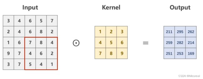
设定对于规格为$1\times W\times H$的原图，利用一个规格为$1\times W^{\prime }\times H^{\prime }$的卷积核进行卷积处理的数乘操作。

则需要从原始数据的左上角开始依次选取与核的规格相同($1\times W^{\prime }\times H^{\prime }$)的输入数据进行数乘操作，并将求得的数值作为一个Output值进行填充。

Patch在原图上进行滑动时，每次只滑动一个像素，即包含重复计算的部分

最后求得的Output的像素矩阵，即是对原图像，在设定的卷积核下的卷积结果，是一个规格为$1\times W^{\prime }\times H^{\prime }$的图像。

多通道卷积

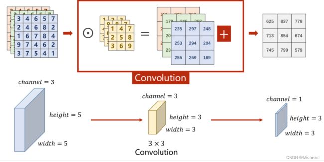
对于多通道图像($N\times W\times H$)，每一个通道是一个单通道的图像（$1\times W\times H$）都要有一个自己的卷积核（$1\times W^{\prime }\times H^{\prime }$）来进行卷积。

对于分别求出来的矩阵，需要再次进行求和才能得到最后的输出矩阵，最终的输出矩阵仍然是一个$1\times W^{\prime }\times H^{\prime }$的 图像。

将平面的图像转为立体的角度即如下图

改进多通道

多通道卷积中，每次只能把$N$个通道转变为1个通道，而无法在通道这个维度进行增加或降低。

因此，为了对通道进行更加灵活的操作，可以将原先$N\times W\times H$的图像，利用不同的卷积核对其多次求卷积，由于每次求卷积之后的输出图像为$1\times W^{\prime }\times H^{\prime }$，若一共求解了$M$次，即可以将此$M$次的求解结果按顺序在通道（Channel）这一维度上进行拼接，以此来形成一个规格为$M\times W^{\prime }\times H^{\prime }$的图像。

总结以及课程代码

1. 每个卷积核的通道数与原通道数一致
2. 卷积核的数量与输出通道数一致
3. 卷积核的大小与图像大小无关

上述中所提到的卷积核，是指的多通道的卷积核，而非前文中提到的二维的。
综上所述为了使下图所表征的过程成立，即若需要使得原本为$n\times widt{h}_{in}\times heigh{t}_{in}$的图像转变为一个$m\times widt{h}_{out}\times heigh{t}_{out}$的图像，可以利用$m$个大小为$n\times kernel\_siz{e}_{width}\times kernel\_siz{e}_{height}$的卷积核。

则在实际操作中，即可抽象为利用一个四维张量作为卷积核，此四维张量的大小为$m\times n\times kernel\_siz{e}_{width}\times kernel\_siz{e}_{height}$

import torch
in_channels, out_channels = 5, 10
width, height = 100, 100

kernel_size = 3 #默认转为3*3，最好用奇数正方形

#在pytorch中的数据处理都是通过batch来实现的
#因此对于C*W*H的三个维度图像，在代码中实际上是一个B（batch）*C*W*H的四个维度的图像
batch_size = 1

#生成一个四维的随机数
input = torch.randn(batch_size, in_channels, width, height)

#Conv2d需要设定，输入输出的通道数以及卷积核尺寸
conv_layer = torch.nn.Conv2d(in_channels, out_channels, kernel_size=kernel_size)

output = conv_layer(input)

print(input.shape)
print(output.shape)
print(conv_layer.weight.shape)

输出结果：

卷积改进

Padding

若对于一个大小为$N\times N$的原图，经过大小为$M\times M$的卷积核卷积后，仍然想要得到一个大小为$N\times N$的图像，则需要对原图进行Padding，即外围填充。

例如，对于一个$5\times 5$的原图，若想使用一个$3\times 3$的卷积核进行卷积，并获得一个同样$5\times 5$的图像，则需要进行Padding，通常外围填充0

input = [3,4,6,5,7,
         2,4,6,8,2,
         1,6,7,8,4,
         9,7,4,6,2,
         3,7,5,4,1]

#将输入变为B*C*W*H
input = torch.Tensor(input).view(1, 1, 5, 5)

#偏置量bias置为false
conv_layer = torch.nn.Conv2d(1, 1, kernel_size=3, padding=1, bias=False)

#将卷积核变为CI*CO*W*H
kernel = torch.Tensor([1,2,3,4,5,6,7,8,9]).view(1, 1, 3, 3)

#将做出来的卷积核张量，赋值给卷积运算中的权重（参与卷积计算）
conv_layer.weight.data = kernel.data

output = conv_layer(input)

print(output)

Stride

本质上即是Batch的步长，在Batch进行移动时，每次移动Stride的距离，以此来有效降低图像的宽度与高度。

例如，对于一个$5\times 5$的原图，若想使用一个$3\times 3$的卷积核进行卷积，并获得一个$2\times 2$的图像，则需要进行Stride，且Stride=2

import torch
input = [3,4,6,5,7,
         2,4,6,8,2,
         1,6,7,8,4,
         9,7,4,6,2,
         3,7,5,4,1]

#将输入变为B*C*W*H
input = torch.Tensor(input).view(1, 1, 5, 5)

#偏置量bias置为false
conv_layer = torch.nn.Conv2d(1, 1, kernel_size=3, stride=2, bias=False)

#将卷积核变为CI*CO*W*H
kernel = torch.Tensor([1,2,3,4,5,6,7,8,9]).view(1, 1, 3, 3)

#将做出来的卷积核张量，赋值给卷积运算中的权重（参与卷积计算）
conv_layer.weight.data = kernel.data

output = conv_layer(input)

print(output)

下采样过程

大池化层（Max Pooling）

对于一个$M\times M$图像而言，通过最大池化层可以有效降低其宽度和高度上的数据量，例如通过一个$N\times N$的最大池化层，即将原图分为若干个$N\times N$大小的子图，并在其中选取最大值填充到输出图中，此时输出图的大小为$\frac{M}{N}\times \frac{M}{N}$ 。

import torch
input = [3,4,6,5,
         2,4,6,8,
         1,6,7,8,
         9,7,4,6]

input = torch.Tensor(input).view(1, 1, 4, 4)

#kernel_size=2 则MaxPooling中的Stride也为2
maxpooling_layer = torch.nn.MaxPool2d(kernel_size=2)

output = maxpooling_layer(input)

print(output)

简单卷积神经网络的实现

class Net(torch.nn.Module):
    def __init__(self):
        super(Net, self).__init__()
        self.conv1 = torch.nn.Conv2d(1, 10, kernel_size=5)
        self.conv2 = torch.nn.Conv2d(10, 20, kernel_size=5)
        self.pooling = torch.nn.MaxPool2d(2)
        self.fc = torch.nn.Linear(320, 10)

    def forward(self, x):
        batch_size = x.size(0)
        x = self.pooling(F.relu(self.conv1(x)))
        x = self.pooling(F.relu(self.conv2(x)))
        x = x.view(batch_size, -1)
        x = self.fc(x)
        return x

课程代码

import torch
from torchvision import transforms
from torchvision import datasets
from torch.utils.data import DataLoader
import torch.nn.functional as F
import torch.optim as optim
 
# prepare dataset
 
batch_size = 64
transform = transforms.Compose([transforms.ToTensor(), transforms.Normalize((0.1307,), (0.3081,))])
 
train_dataset = datasets.MNIST(root='../dataset/mnist/', train=True, download=True, transform=transform)
train_loader = DataLoader(train_dataset, shuffle=True, batch_size=batch_size)
test_dataset = datasets.MNIST(root='../dataset/mnist/', train=False, download=True, transform=transform)
test_loader = DataLoader(test_dataset, shuffle=False, batch_size=batch_size)
 
# design model using class
 
class Net(torch.nn.Module):
    def __init__(self):
        super(Net, self).__init__()
        self.conv1 = torch.nn.Conv2d(1, 10, kernel_size=5)
        self.conv2 = torch.nn.Conv2d(10, 20, kernel_size=5)
        self.pooling = torch.nn.MaxPool2d(2)
        self.fc = torch.nn.Linear(320, 10)
 
 
    def forward(self, x):
        # flatten data from (n,1,28,28) to (n, 784)
        batch_size = x.size(0)
        x = F.relu(self.pooling(self.conv1(x)))
        x = F.relu(self.pooling(self.conv2(x)))
        x = x.view(batch_size, -1) # -1 此处自动算出的是320
        x = self.fc(x)
 
        return x
 
 
model = Net()
 
# construct loss and optimizer
criterion = torch.nn.CrossEntropyLoss()
optimizer = optim.SGD(model.parameters(), lr=0.01, momentum=0.5)
 
# training cycle forward, backward, update
 
 
def train(epoch):
    running_loss = 0.0
    for batch_idx, data in enumerate(train_loader, 0):
        inputs, target = data
        optimizer.zero_grad()
 
        outputs = model(inputs)
        loss = criterion(outputs, target)
        loss.backward()
        optimizer.step()
 
        running_loss += loss.item()
        if batch_idx % 300 == 299:
            print('[%d, %5d] loss: %.3f' % (epoch+1, batch_idx+1, running_loss/300))
            running_loss = 0.0
 
 
def test():
    correct = 0
    total = 0
    with torch.no_grad():
        for data in test_loader:
            images, labels = data
            outputs = model(images)
            _, predicted = torch.max(outputs.data, dim=1)
            total += labels.size(0)
            correct += (predicted == labels).sum().item()
    print('accuracy on test set: %d %% ' % (100*correct/total))
 
 
if __name__ == '__main__':
    for epoch in range(10):
        train(epoch)
        test()