【无标题】

RDD

• Resilient Distributed Datasets
  • A distributed memory abstraction enabling in-memory computations on large clusters in a fault-tolerant manner
  • The primary data abstraction in Spark enabling operations on collection of elements in parallel
• R: recompute missing partitions due to node failures
• D: data distributed on multiple nodes in a cluster
• D: a collection of partitioned elements (datasets)

RDD Traits
• In-Memory: data inside RDD is stored in memory as much (size) and long (time) as possible
• Immutable (read-only): no change after creation, only transformed using transformations to new RDDs
• Lazily evaluated: RDD data not available/transformed until an action is executed that triggers the execution
• Parallel: process data in parallel
• Partitioned: the data in a RDD is partitioned and then distributed across nodes in a cluster
• Cacheable: hold all the data in a persistent “storage” like memory (the most preferred) or disk (the least preferred)

RDD Operations
• Transformation: takes an RDD and returns a new RDD but nothing gets evaluated / computed
• Action: all the data processing queries are computed (evaluated ) and the result value is returned

RDD Workflow
• Create an RDD from a data source, e.g. RDD or file
• Apply transformations to an RDD, e.g., map, filter
• Apply actions to an RDD, e.g., collect, count
• Users to control 1) persistence, 2) partitioning

Creating RDDs
• Parallelize existing Python collections (lists)
• Transform existing RDDs
• Create from (HDFS, text, Amazon S3) files
• sc APIs: sc.parallelize, sc.hadoopFile, sc.textFile

Shared Variables (for Cluster)
• Variables are distributed to workers via closures
• When a function is executed on a cluster node, it works on separate copies of those variables that are not shared across workers

• Iterative or single jobs with large global variables
  • Problem: inefficient to send large data with each iteration
  • Solution: Broadcast variables (keep rather than ship)
• Counting events that occur during job execution
  • Problem: Closures are one way driver —> worker
  • Solution: Accumulators (only “added” to, e.g. sums/counters)

Typed and untyped APIs
Typed:
Scala,Java
untyped:
Scala,Python,R*

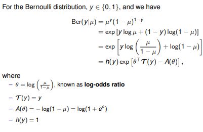
Bernoulli distribution

A Bernoulli random variable can only take two possible values

A Bernoulli distribution is a probability distribution for Y , expressed as

The target value y follows a Bernoulli distribution
In logistic regression, the probability μ(x) is given as，/where σ(z) is known as the sigmoid function, and w is the coefficient vector to learn.

Newton’s algorithm

It derives a faster optimisation algorithm by taking the curvature of the space (i.e., the Hessian) into account.

Quasi-Newton methods
In place of the true Hessian Hk , they use an approximation Bk , which is updated after each
step to take account of the additional knowledge gained during the step
BFGS formula for Hk：

This is a rank-two update to the matrix, and ensures that the matrix remains positive definite

Limited memory BFGS (L-BFGS)

regularisation

It refers to a technique used for preventing overfitting in a predictive model.
It consists in adding a term (a regulariser) to the objective function that encourages simpler solutions
L(w) = NLL(w) + λR(w)，where R(w) is the regularisation term and λ the regularisation parameter
If λ = 0, we get L(w) = NLL(w)

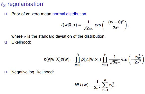
l2 regularisation

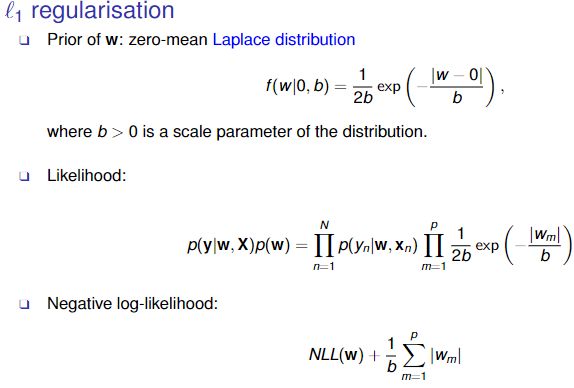
l1 regularisation

elastic net regularisation

SGD

In stochastic gradient descent (SGD), the gradient gk is computed using a subset of the instances available.

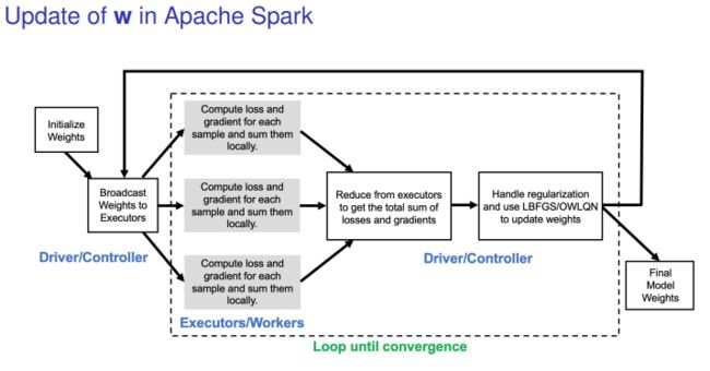
controller: broadcast weights to executors
executors: compute loss and gradient for each sample and sum them locally
driver: reduce from executors to get the local sum of losses and gradients
driver: handle regulaization and use LBFGS to update weights

regression

Linear regression, y → continuous
Logistic regression, y → categorical (binary)

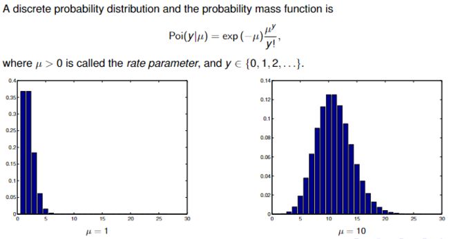
Poisson distribution

Poisson regression

Generalised form:

exponential family

h(y) is a scaling constant, often 1
θ are known as the natural parameters or canonical parameters
T (y) ∈ Rd is called a vector of sufficient statistics
Z (θ) is known as the partition function

A(θ) is called the log partition function or cumulant function
If T (y) = y, we say it is a natural exponential family

the exponential family is important is because It can be shown that the exponential family is the only family of distributions with finite-sized
sufficient statistics.
The exponential family is the only family of distributions for which conjugate priors exist.
The exponential family is at the core of generalised linear models.

g^−1() is the mean function. g() is the link function
这是一些我估计背不下来的公式，考试考到了就随天命吧
Bernoulli

univariate Gaussian distribution

---

In linear regression, the response variable follows a normal distribution,

---

In logistic regression, the response variable follows a Bernoulli distribution,

---

In Poisson regression, the response variable follows a Poisson distribution,

---

A least squares (LS) problem refers to:

It can be shown that the vector w that minimises LS(w) is given as

---

A weighted least squares (WLS) problem refers to

It can be shown that the vector w that minimises WLS(w) is given as

GeneralizedLinearRegression()

If your ‘family’ is Gaussian and the link function is the ‘identity’, your model is just equivalent to linear regression
If your ‘family’ is Binomial and the link function is ‘logit’, your model is equivalent to logistic regression

RecSys

Recommender Systems (RecSys)
• Predict relevant items for a user, in a given context
• Predict to what extent these items are relevant
• A ranking task (searching as well)
• Implicit, targeted, intelligent advertisement
• Effective, popular marketing

Two Classes of RecSys
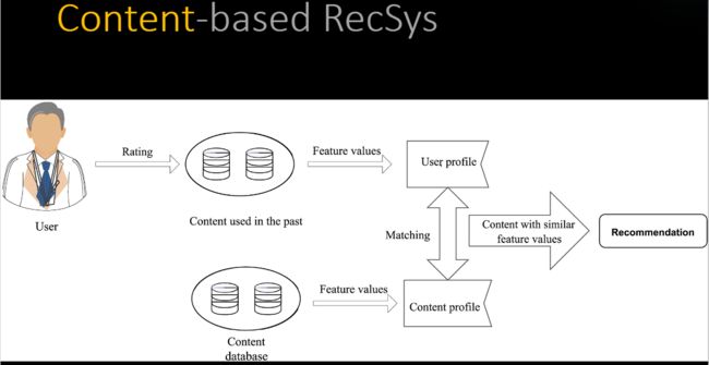
• Content-based recommender systems
• Collaborative filtering recommender systems

Collaborative Filtering

• Information filtering based on past records
  • Electronic word of mouth marketing
  • Turn visitors into customers (e-Salesman)
• Components
  • Users (customers): who provide ratings
  • Items (products): to be rated
  • Ratings (interest): core data

Objective: predict how well a user will like an unrated item, given past ratings for a community of users

• Explicit (direct): users indicate levels of interest
  • Most accurate descriptions of a user’s preference
  • Challenging in collecting data
• Implicit (indirect): observing user behavior
  • Can be collected with little or no cost to user
  • Ratings inference may be imprecise

Rating Scales

• Scalar ratings
  • Numerical scales
  • 1-5, 1-7, etc.
• Binary ratings
  • Agree/Disagree, Good/Bad, etc.
• Unary ratings
  • Presence/absence of an event, e.g., purchase/browsing history, search patterns, mouse movements
  • No info about the opposite ≠ 0

Collaborative Filtering Methods

• Memory-based: predict using past ratings directly
  • Weighted ratings given by other similar users
  • User-based & item-based (non-ML)
• Model-based: model users based on past ratings
  • Predict ratings using the learned model
  

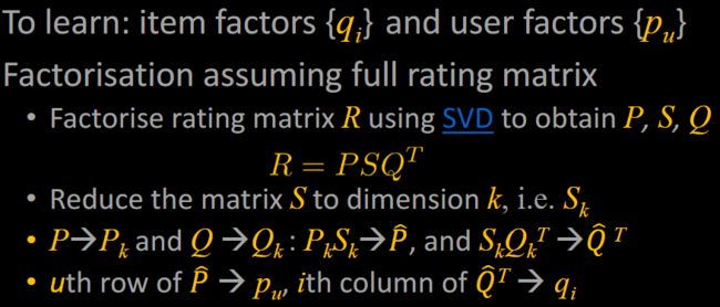
Matrix Factorisation (MF) for CF

• Characterise items/users by vectors of factors learned from the rating matrix user x item
• High correlation between item and user factors -> good recommendation
• Flexibility: incorporate implicit feedback, temporal effects, and confidence levels

Basic MF Model

Map users & items to a joint latent factor space of dimensionality k
• Item i -> vector qi: the extent to which the item possesses those k factors
• User u: vector pu: the extent of interest the user has on those k factors

User-item interactions: the user’s overall interest in the item’s characteristics

MF with Missing Values

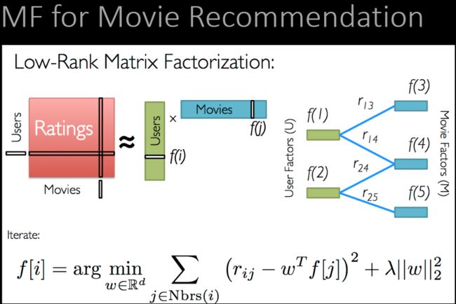
Modelling directly the observed ratings only
• Avoid overfitting through a regularised model
• Minimize the regularised squared error on the set of known ratings to learn the factor vectors p u and qi



spark里用ALS 这个API

Kmeans

Hierarchical Clustering

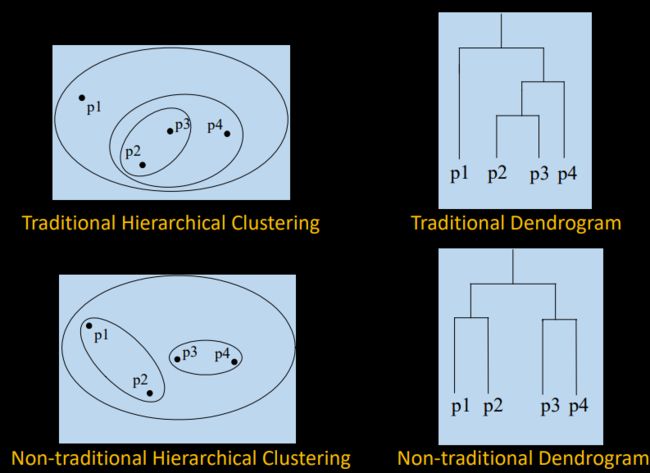
Traditional Hierarchical Clustering
Non-traditional Hierarchical Clustering
Traditional Dendrogram
Non-traditional Dendrogram

Hierarchical: nested clusters as a hierarchical tree
• Each node (cluster) in the tree (except for the leaf nodes) is the union of its children (subclusters)
• The root of the tree  the cluster containing all data points

Partitional: non-overlapping clusters
• Each data point is in exactly one cluster

k-means Clustering

• A centre-based, partitional clustering approach
• Input: a set of n data points X={x1, x2, …, xn} and the number of clusters k
• For a set C={c1, c2, …, ck} of cluster centres, define the Sum of Squared Error (SSE) as
d(x,C): distance from x to the closest centre in C
Goal: find C centres minimising SSE

Lloyd Algorithm for k-means
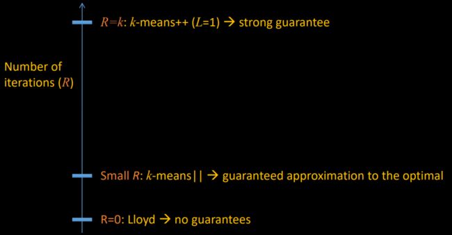
Start with k centres {c1, c2, …, ck} chosen uniformly at random from data points

K++

Key idea: spread out the centres
Choose the first centre c1 uniformly at random
Choose ci to be equal to a data point x0 sampled from the distribution
k-means++ limitations
• Needs k passes over the data for initilisation
• In big data applications, k is typically large (e.g., 1000) ,so that not scalable

K2

Choose the oversampling factor L>1
Initialise C to an arbitrary set of points
Cluster the intermediate centres in C using k-means++

Benefits over k-means++
• Less susceptible to noisy outliers
• More reduction in the number of Lloyd iterations

PCA

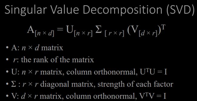
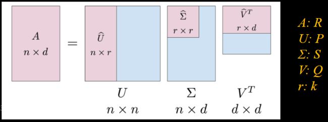
Singular Value Decomposition

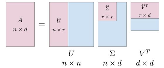
SVD gives
Eigen-decomposition gives
U, V, W: orthonormal
Σ, Λ: diagonal

U: document-to-concept similarity matrix
V: term-to-concept similarity matrix
Σ: its diagonal elements : strength of each concept

Software Development Life Cycle

Phased Development
• Reduce cycle time, deliver in pieces, let users have some functionality while developing the rest
Two or more systems in parallel
• The operational/production system in use by customers
• The development system to replace the current release

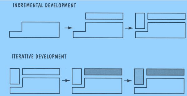
Iterative/Incremental Development

• Incremental: partition a system by functionality
  • Early release: small, functional subsystem
  • Later releases: add functionality
• Iterative: improve overall system in each release
  

Lifecycle Phases

• Inception: rationale, scope, and vision
• Elaboration: “Design/Details”
detailed requirements and high-level analysis/design
• Construction – “Do it”
build software in increments, tested and integrated,each satisfying a subset of the requirements
• Transition – “Deploy it”
beta testing, performance tuning, and user training

decision tree

A decision tree consists of:
▪ A root node (or starting node)
▪ Interior nodes
▪ Leaf nodes (or terminating nodes)
Each of the non-leaf nodes (root and interior) in the tree specifies a test to be carried out on one of the query’s descriptive features
Each of the leaf nodes specifies a predicted classification or predicted regression value for the query

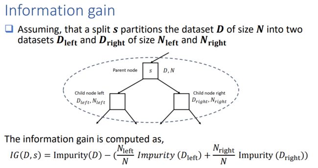
Best split
The best split maximizes the information gain at a tree node
The split chosen at each tree node is chosen from the set,arg max (, )
Here, (, ) is the information gain when split is applied to dataset

Categorical features

Say we have a categorical feature that can take M unordered values, It can be shown there are 2^(−1) − 1 possible partitions of the M values into two groups
As an example, consider the feature weather that takes values [spring, summer, autumn, winter], We would then have 7 possible partitions of two groups.

In Spark, for multiclass classification, all 2^(−1) − 1 possible split are used whenever possible, when that value is greater than the maxBins parameter, Spark uses a heuristic method similar to the method used for binary classification and regression

PLANET: horizontal partitioning

PLANET is the standard algorithm to train a decision in a distributed dataset or horizontal partitioning
Horizontal partitioning refers to the fact that each worker will receive a subset of the n instances or row vectors

Algorithm to compute ∗ in a distributed fashion,
start by assuming the depth of the tree is fixed to D,
At iteration t,
▪ the algorithm computes the optimal splits for all the nodes on the level t of the tree
▪ there is a single round trip of communication between the master and the workers

Each tree node i is split as follows

1. The j-th worker locally computes sufficient statistics () for all ∈
2. Each worker communicates all statistics () to the master (Bp in total)
3. The master computes the best split ∗
4. The master broadcasts ∗ to the workers, who update their local states to keep track of which instances are assigned to which child nodes

Bagging

In bagging (or bootstrap aggregating) each model in the ensemble is trained on a random sample of the dataset known as bootstrap samples
Each random sample is the same size as the dataset and sampling with replacement is used
Hence, every bootstrap sample will be missing some of the instance from the dataset. Consequently
▪ Each bootstrap sample will be different
▪ Therefore, models trained on different bootstrap samples will also be different

When bagging is used with decision trees, each boostrap sample only uses a randomly selected subset of the descriptive features in the dataset (This is known as subspace sampling ),The combination of bagging, subspace sampling and decision trees is known as a random forest model

Boosting

❑Boosting works by iteratively creating models and adding them to the ensemble
❑The iteration stops when a predefined number of models have been added
❑When we use boosting each new model added to the ensemble is biased to pay more attention to instance that previous models missclassified
❑This is done by incrementally adapting the dataset used to train the models. To do this, we use a weighted dataset
Each instance has an associated weight, w ≥ 0
Initially set to 1/ where is the number of instances in the dataset
After each model is added to the ensemble, it is tested on the training data:
▪ Weights of the instances that the model accurately predicts are decreased
▪ Weights of the instances that the model predicts incorrectly are increased

These weights are used as a distribution over which the dataset is sampled to create a replicated training set (Replication of an instance is proportional to its weight)