作者:taoyan
链接:https://www.jianshu.com/p/b7274afff14f
来源:
仅用来备份学习查找,让删随时删!!!
#先加载包
library(ggpubr)
#加载数据集ToothGrowth
data("ToothGrowth")
head(ToothGrowth)
##    len  supp  dose
## 1  4.2   VC   0.5
## 2  11.5  VC   0.5
## 3  7.3   VC   0.5
## 4  5.8   VC   0.5
## 5  6.4   VC   0.5
## 6  10.0  VC   0.5
比较方法
R中常用的比较方法主要有下面几种:
| 方法 | R函数 | 描述 |
|---|---|---|
| T-test | t.test() | 比较两组(参数) |
| Wilcoxon test | wilcox.test() | 比较两组(非参数) |
| ANOVA | aov()或anova() | 比较多组(参数) |
| Kruskal-Wallis | kruskal.test() | 比较多组(非参数) |
各种比较方法后续有时间一一讲解。
添加p-value
主要利用ggpubr包中的两个函数:
-
compare_means():可以进行一组或多组间的比较 -
stat_compare_mean():自动添加p-value、显著性标记到ggplot图中
compare_means()函数
该函数主要用用法如下:
compare_means(formula, data, method = "wilcox.test", paired = FALSE,
  group.by = NULL, ref.group = NULL, ...)
注释:
-
formula:形如x~group,其中x是数值型变量,group是因子,可以是一个或者多个 -
data:数据集 -
method:比较的方法,默认为"wilcox.test", 其他可选方法为:"t.test"、"anova"、"kruskal.test" -
paired:是否要进行paired test(TRUEorFALSE) -
group_by: 比较时是否要进行分组 -
ref.group: 是否需要指定参考组
stat_compare_means()函数
主要用法:
stat_compare_means(mapping = NULL, comparisons = NULL hide.ns = FALSE,
                   label = NULL,  label.x = NULL, label.y = NULL,  ...)
注释:
-
mapping:由aes()创建的一套美学映射 -
comparisons:指定需要进行比较以及添加p-value、显著性标记的组 -
hide.ns:是否要显示显著性标记ns -
label:显著性标记的类型,可选项为:p.signif(显著性标记)、p.format(显示p-value) -
label.x、label.y:显著性标签调整 - ...:其他参数
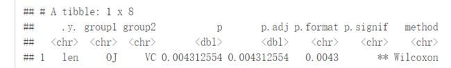
比较独立的两组
compare_means(len~supp, data=ToothGrowth)
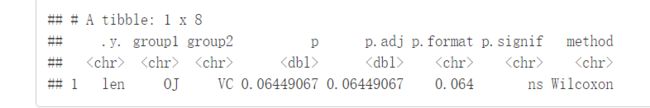
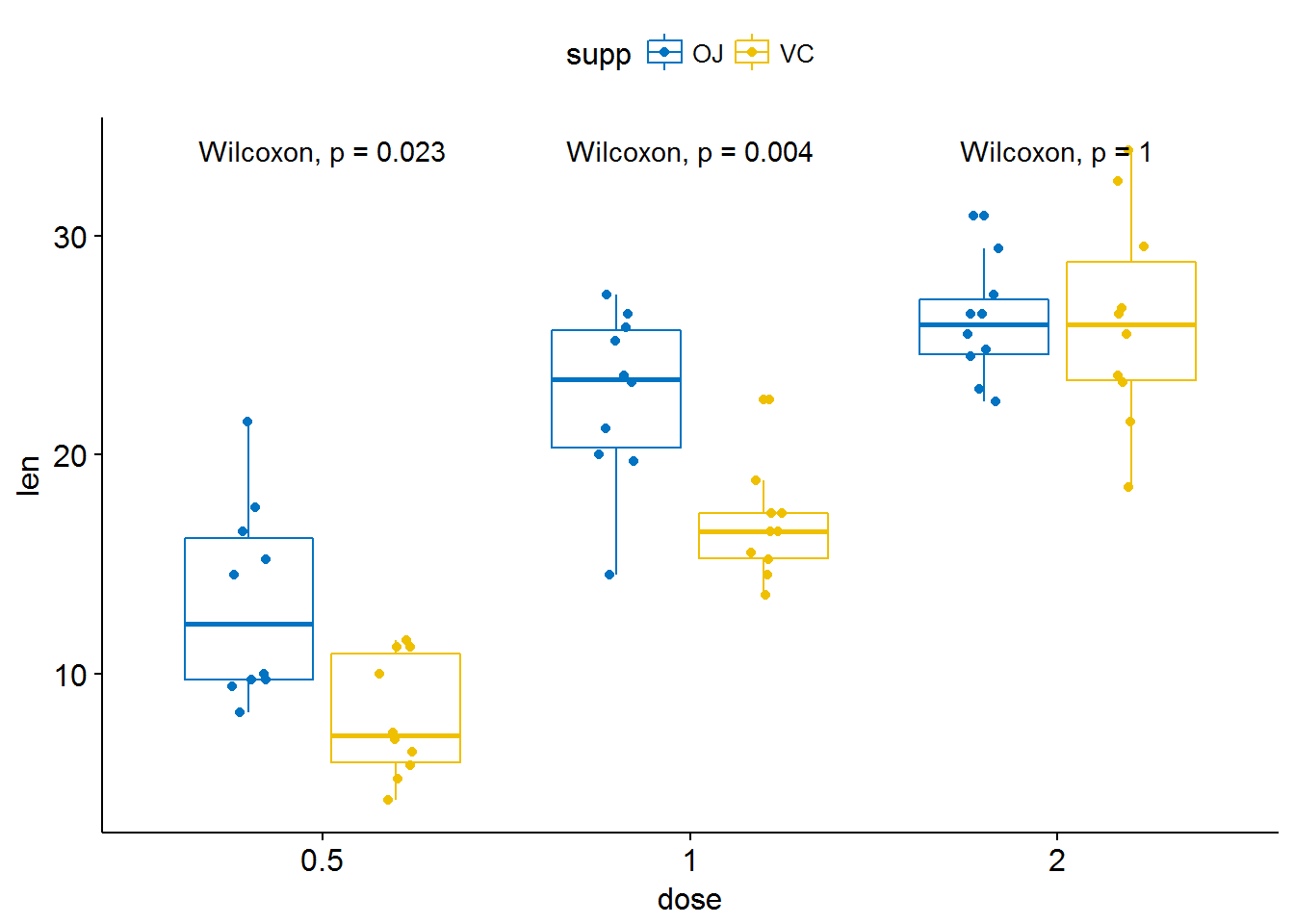
结果解释:
-
.y:测试中使用的y变量 -
p:p-value -
p.adj:调整后的p-value。默认为p.adjust.method="holm" -
p.format:四舍五入后的p-value -
p.signif:显著性水平 -
method:用于统计检验的方法
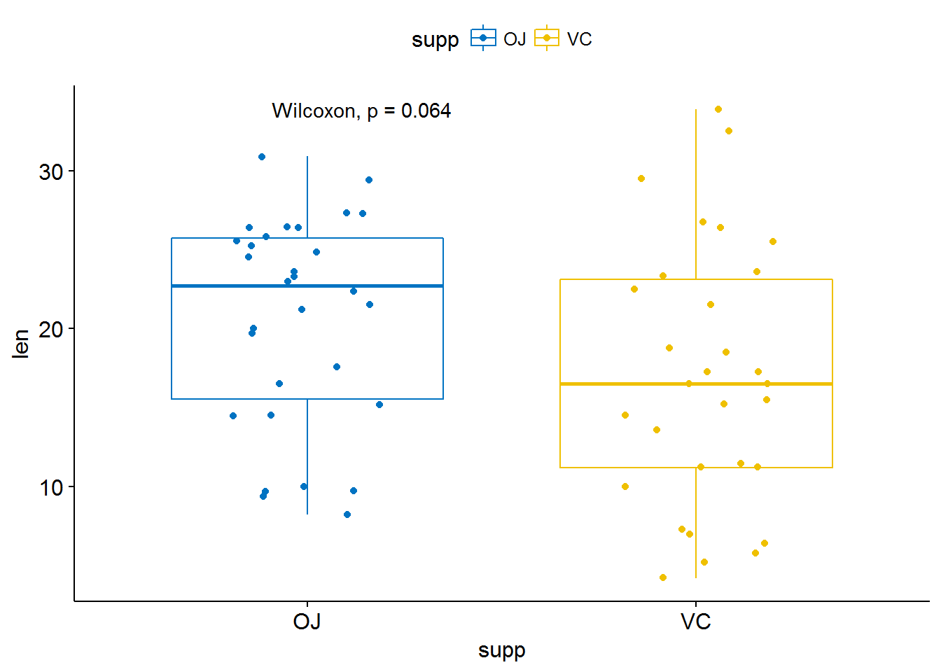
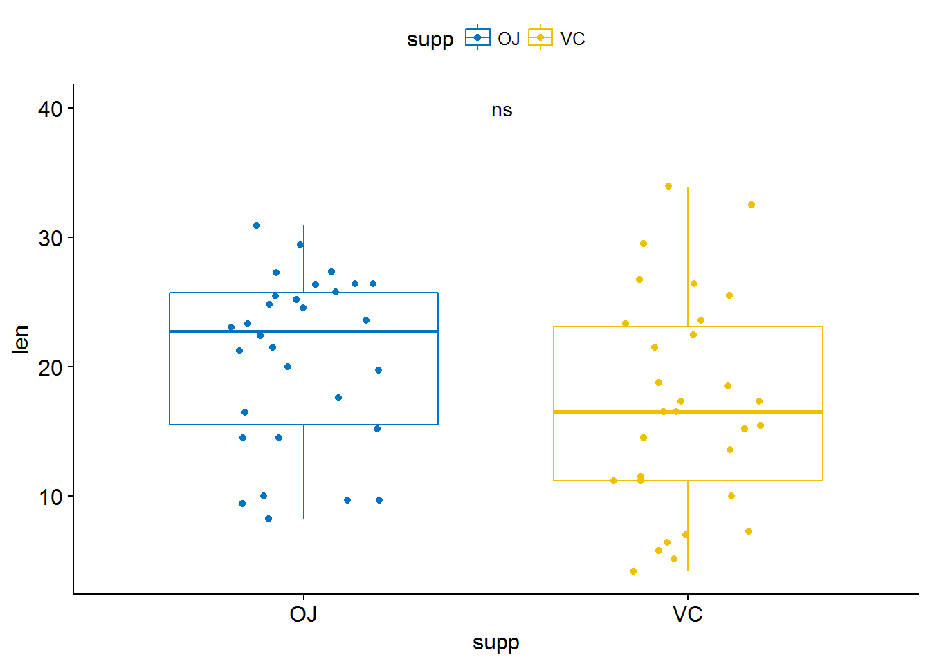
绘制箱线图
p <- ggboxplot(ToothGrowth, x="supp", y="len", color = "supp",
palette = "jco", add = "jitter")#添加p-valuep+stat_compare_means()
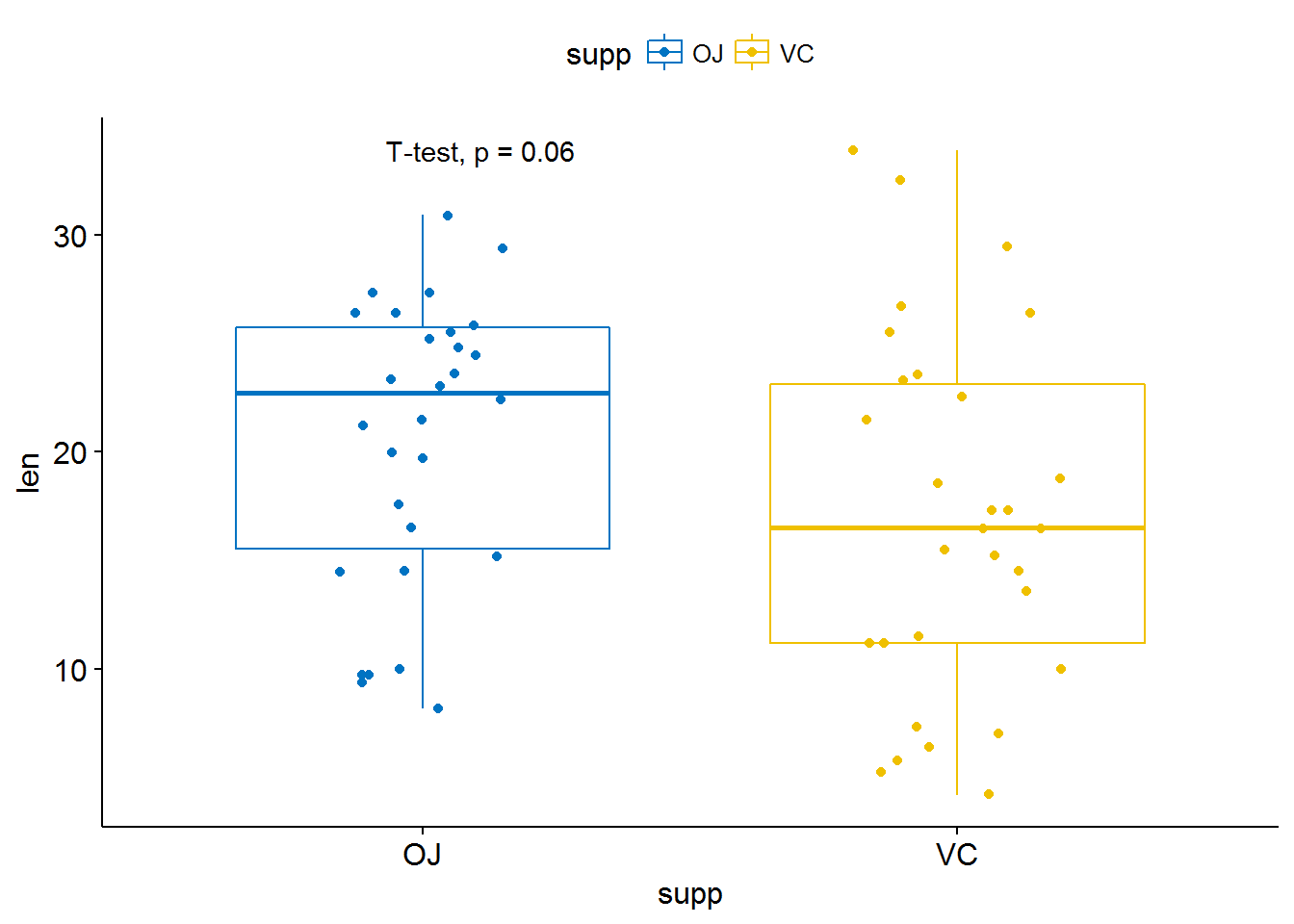
#使用其他统计检验方法
p+stat_compare_means(method = "t.test")
上述显著性标记可以通过label.x、label.y、hjust及vjust来调整
显著性标记可以通过aes()映射来更改:
-
aes(label=..p.format..)或aes(lebel=paste0("p=",..p.format..)):只显示p-value,不显示统计检验方法 -
aes(label=..p.signif..):仅显示显著性水平 -
aes(label=paste0(..method..,"\n", "p=",..p.format..)):p-value与显著性水平分行显示
举个栗子:
p+stat_compare_means(aes(label=..p.signif..), label.x = 1.5, label.y = 40)
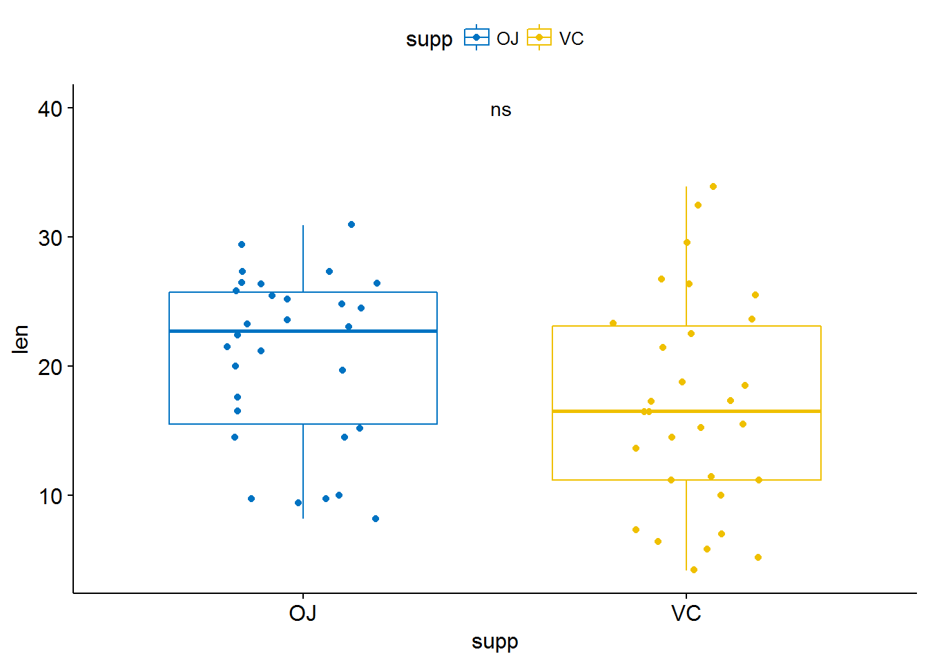
也可以将标签指定为字符向量,不要映射,只需将p.signif两端的..去掉即可
p+stat_compare_means(label = "p.signif", label.x = 1.5, label.y = 40)
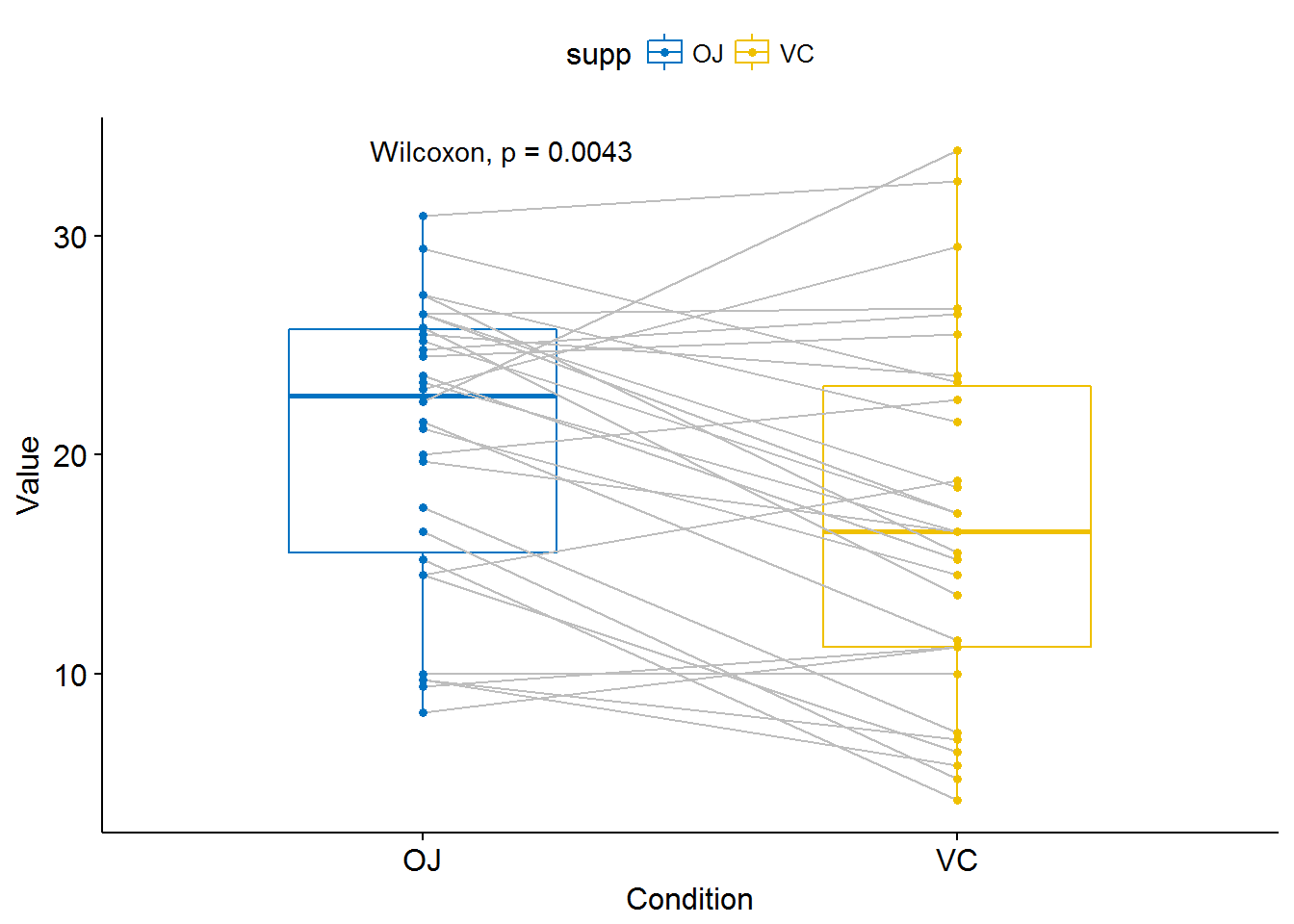
比较两个paired sample
compare_means(len~supp, data=ToothGrowth, paired = TRUE)
利用ggpaired()进行可视化
ggpaired(ToothGrowth, x="supp", y="len", color = "supp", line.color = "gray",
line.size = 0.4, palette = "jco")+ stat_compare_means(paired = TRUE)
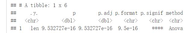
多组比较
Global test
compare_means(len~dose, data=ToothGrowth, method = "anova")
可视化
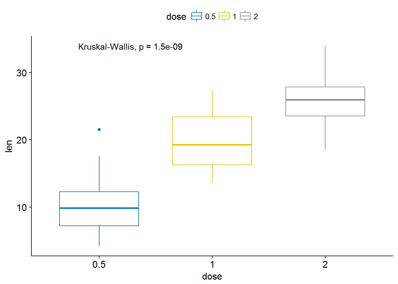
ggboxplot(ToothGrowth, x="dose", y="len", color = "dose", palette = "jco")+
stat_compare_means()
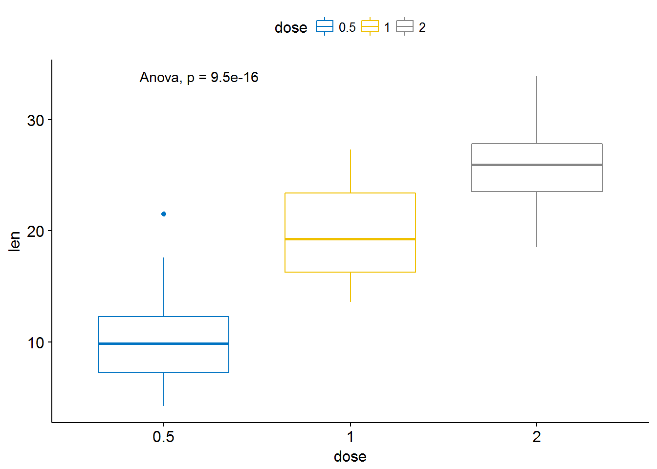
#使用其他的方法
ggboxplot(ToothGrowth, x="dose", y="len", color = "dose", palette = "jco")+
stat_compare_means(method = "anova")
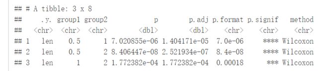
Pairwise comparisons:如果分组变量中包含两个以上的水平,那么会自动进行pairwise test,默认方法为"wilcox.test"
compare_means(len~dose, data=ToothGrowth)
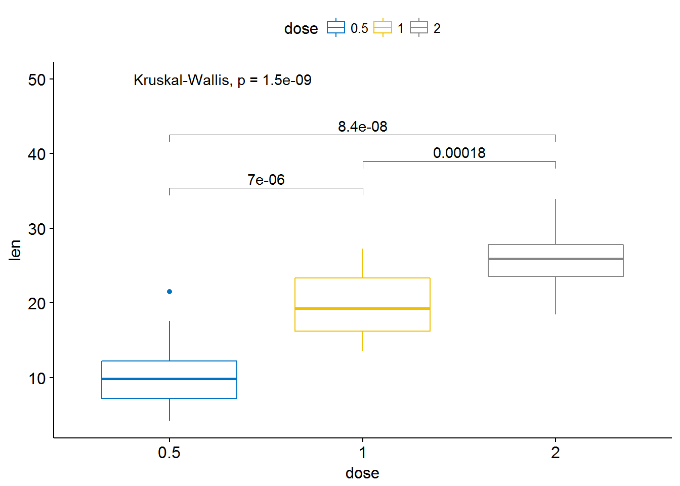
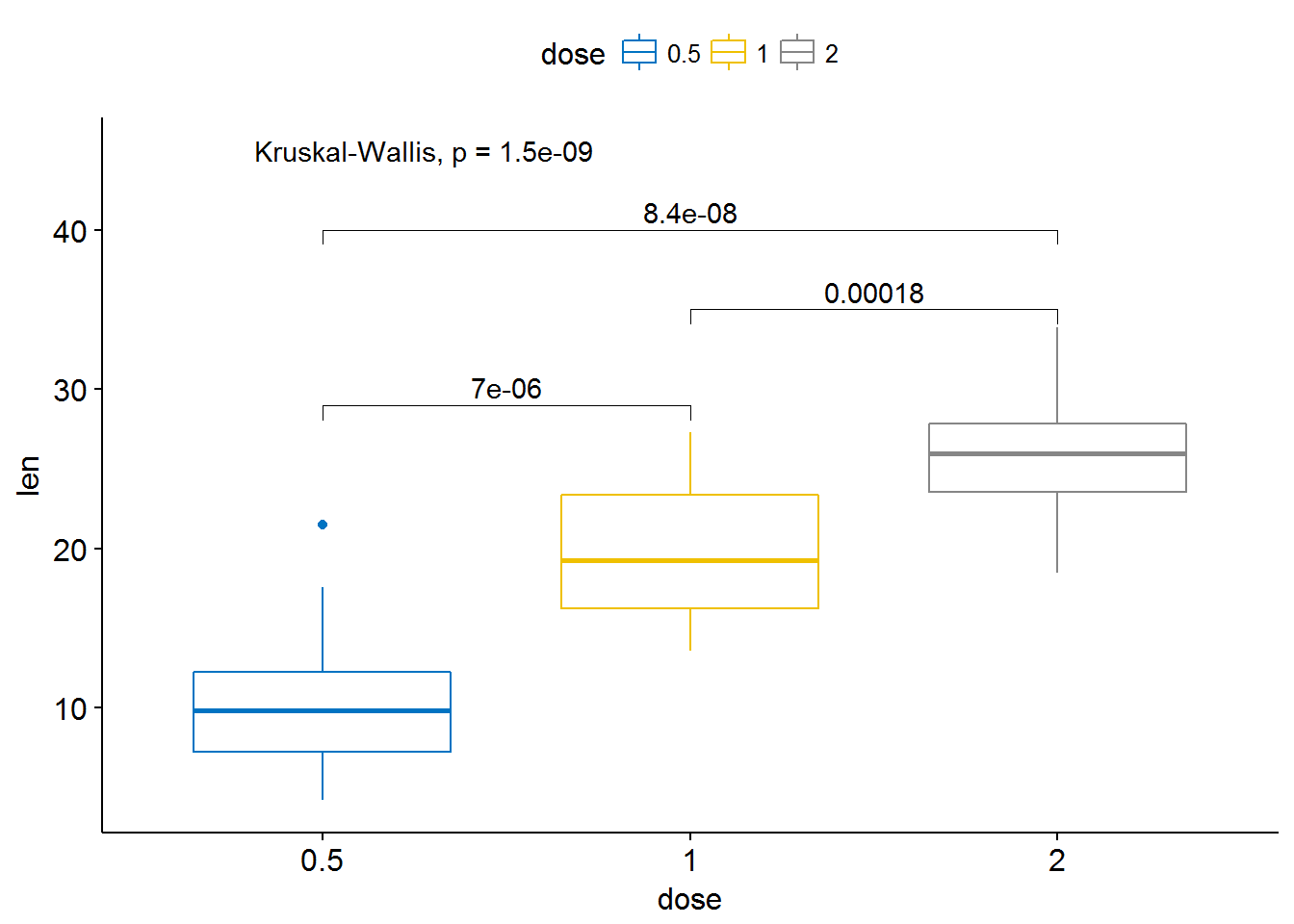
#可以指定比较哪些组
my_comparisons <- list(c("0.5", "1"), c("1", "2"), c("0.5", "2"))
ggboxplot(ToothGrowth, x="dose", y="len", color = "dose",palette = "jco")+
stat_compare_means(comparisons=my_comparisons)+ # Add pairwise
comparisons p-value stat_compare_means(label.y = 50) # Add global p-value
可以通过修改参数label.y来更改标签的位置
ggboxplot(ToothGrowth, x="dose", y="len", color = "dose",palette = "jco")+
stat_compare_means(comparisons=my_comparisons, label.y = c(29, 35, 40))+ # Add pairwise comparisons p-value
stat_compare_means(label.y = 45) # Add global p-value
至于通过添加线条来连接比较的两组,这一功能已由包ggsignif实现
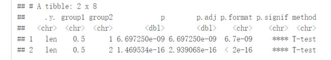
##设定参考组
compare_means(len~dose, data=ToothGrowth, ref.group = "0.5",  #以dose=0.5组为参考组
method = "t.test" )
#可视化
ggboxplot(ToothGrowth, x="dose", y="len", color = "dose", palette = "jco")+
stat_compare_means(method = "anova", label.y = 40)+ # Add global p-value
stat_compare_means(label = "p.signif", method = "t.test", ref.group = "0.5") # Pairwise comparison against reference
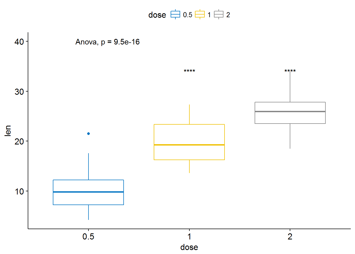
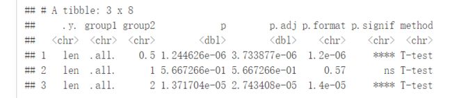
参考组也可以设置为.all.即所有的平均值
compare_means(len~dose, data=ToothGrowth, ref.group = ".all.", method = "t.test")
#可视化
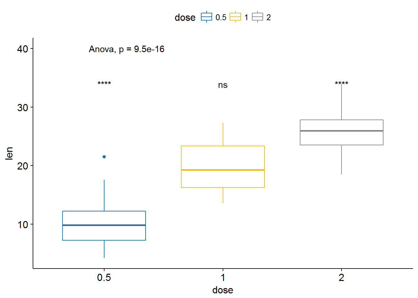
ggboxplot(ToothGrowth, x="dose", y="len", color = "dose", palette = "jco")+
stat_compare_means(method = "anova", label.y = 40)+# Add global p-value
stat_compare_means(label = "p.signif", method = "t.test",
ref.group = ".all.")#Pairwise comparison against all
接下来利用survminer包中的数据集myeloma来讲解一下为什么有时候我们需要将ref.group设置为.all.
library(survminer)#没安装的先安装再加载
data("myeloma")
head(myeloma)
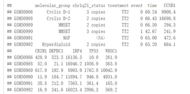
我们将根据患者的分组来绘制DEPDC1基因的表达谱,看不同组之间是否存在显著性的差异,我们可以在7组之间进行比较,但是这样的话组间比较的组合就太多了,因此我们可以将7组中每一组与全部平均值进行比较,看看DEPDC1基因在不同的组中是否过表达还是低表达。
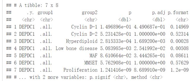
compare_means(DEPDC1~molecular_group, data = myeloma, ref.group = ".all.", method = "t.test")
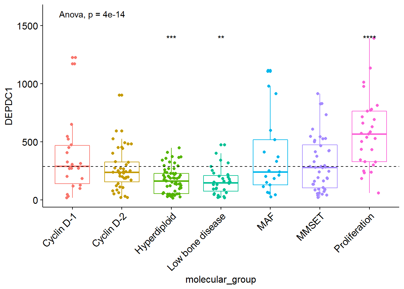
#可视化DEPDC1基因表达谱
ggboxplot(myeloma, x="molecular_group", y="DEPDC1",
color = "molecular_group", add = "jitter", legend="none")+
rotate_x_text(angle = 45)+
geom_hline(yintercept = mean(myeloma$DEPDC1), linetype=2)+# Add horizontal line at base mean
stat_compare_means(method = "anova", label.y = 1600)+ # Add global annova p-value
stat_compare_means(label = "p.signif", method = "t.test", ref.group = ".all.")# Pairwise comparison against all

从图中可以看出,DEPDC1基因在Proliferation组中显著性地过表达,而在Hyperdiploid和Low bone disease显著性地低表达
我们也可以将非显著性标记ns去掉,只需要将参数hide.ns=TRUE
ggboxplot(myeloma, x="molecular_group", y="DEPDC1",
color = "molecular_group", add = "jitter", legend="none")+
rotate_x_text(angle = 45)+
geom_hline(yintercept = mean(myeloma$DEPDC1), linetype=2)+# Add horizontal line at base mean
stat_compare_means(method = "anova", label.y = 1600)+ # Add global annova p-value
stat_compare_means(label = "p.signif", method = "t.test", ref.group = ".all.", hide.ns = TRUE)# Pairwise comparison against all
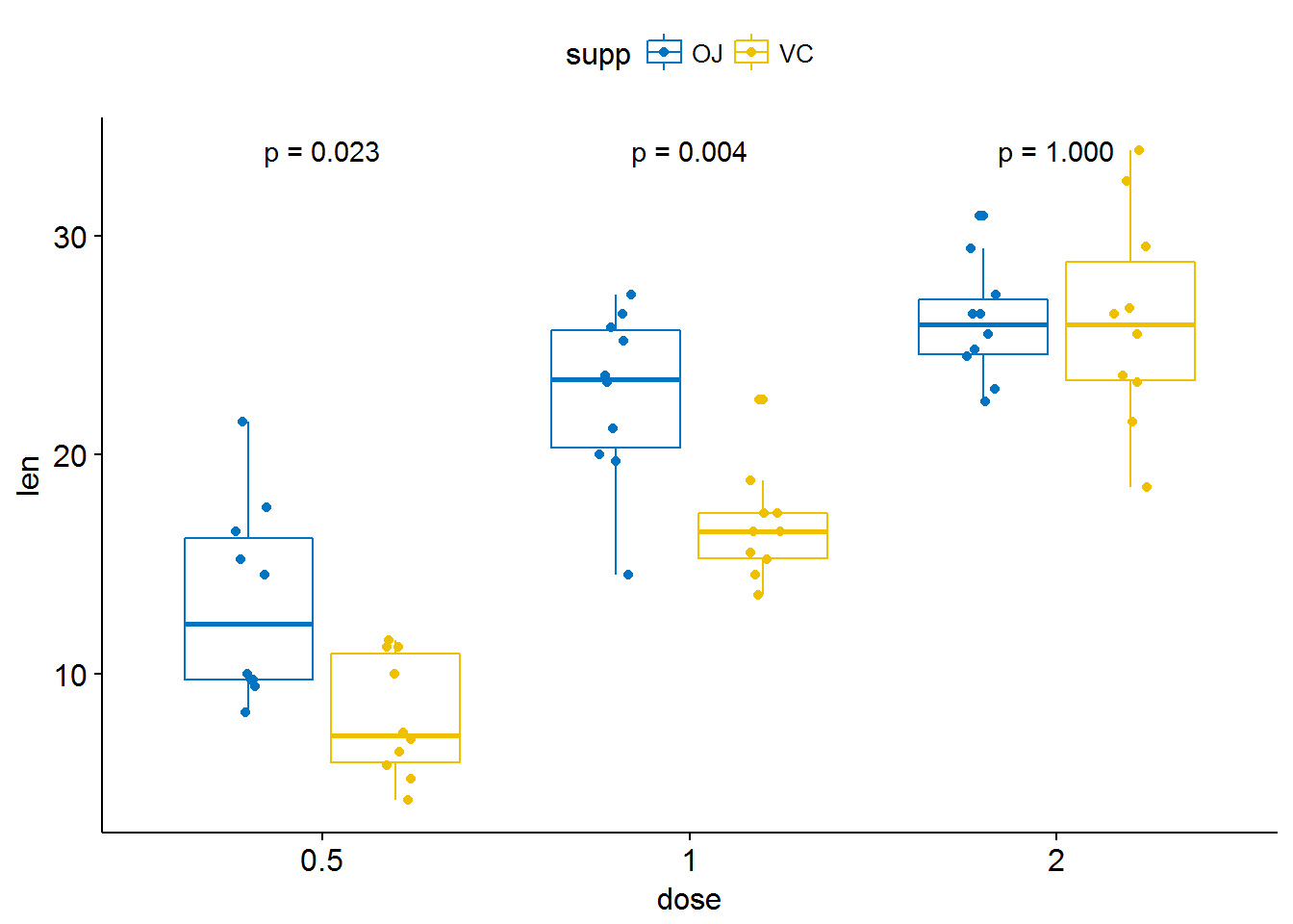
多个分组变量
按另一个变量进行分组之后进行统计检验,比如按变量dose进行分组:
compare_means(len~supp, data=ToothGrowth, group.by = "dose")
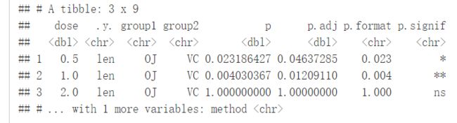
#可视化
p <- ggboxplot(ToothGrowth, x="supp", y="len", color = "supp",
palette = "jco", add = "jitter", facet.by = "dose", short.panel.labs = FALSE)#按dose进行分面
#label只绘制
p-valuep+stat_compare_means(label = "p.format")
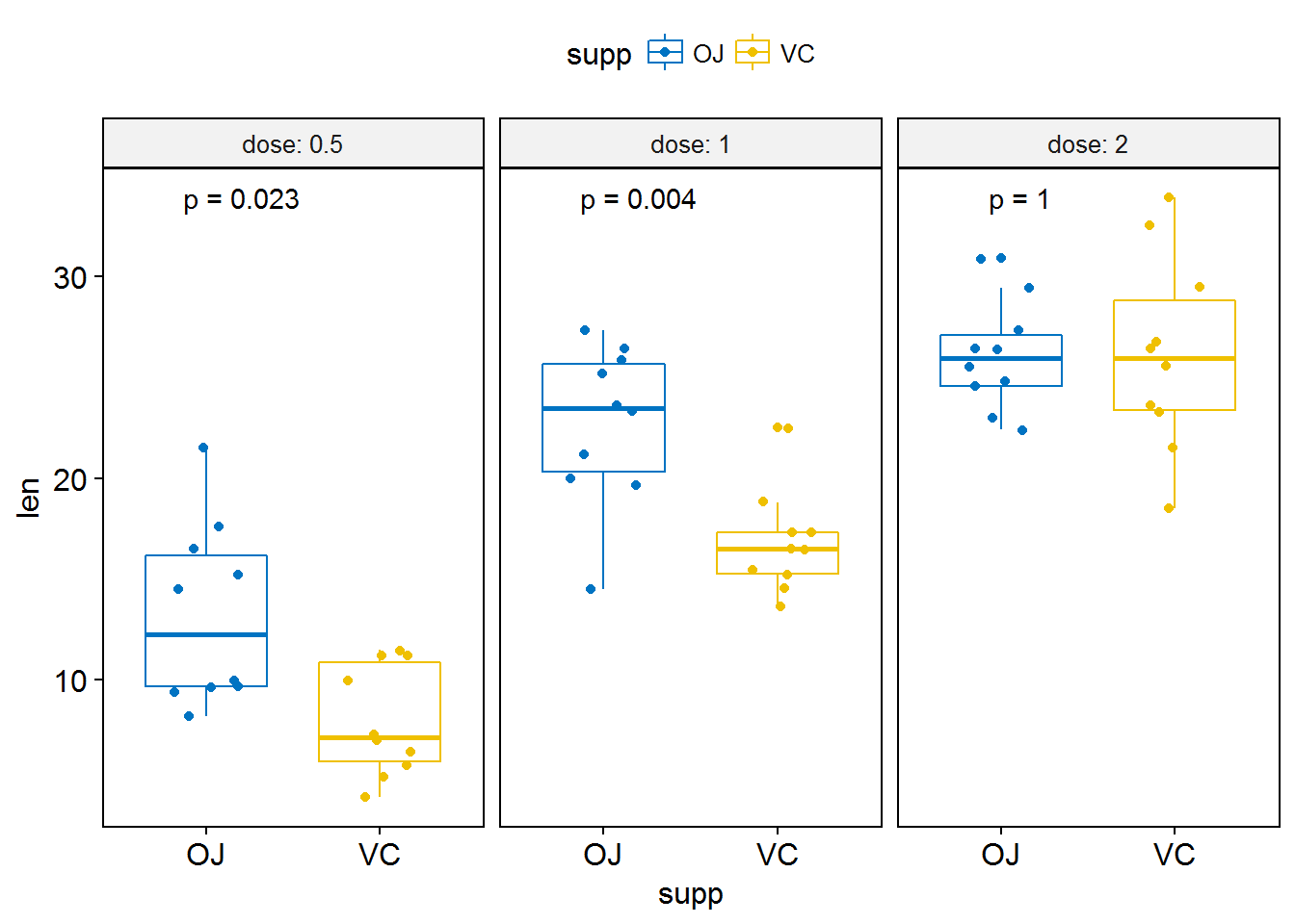
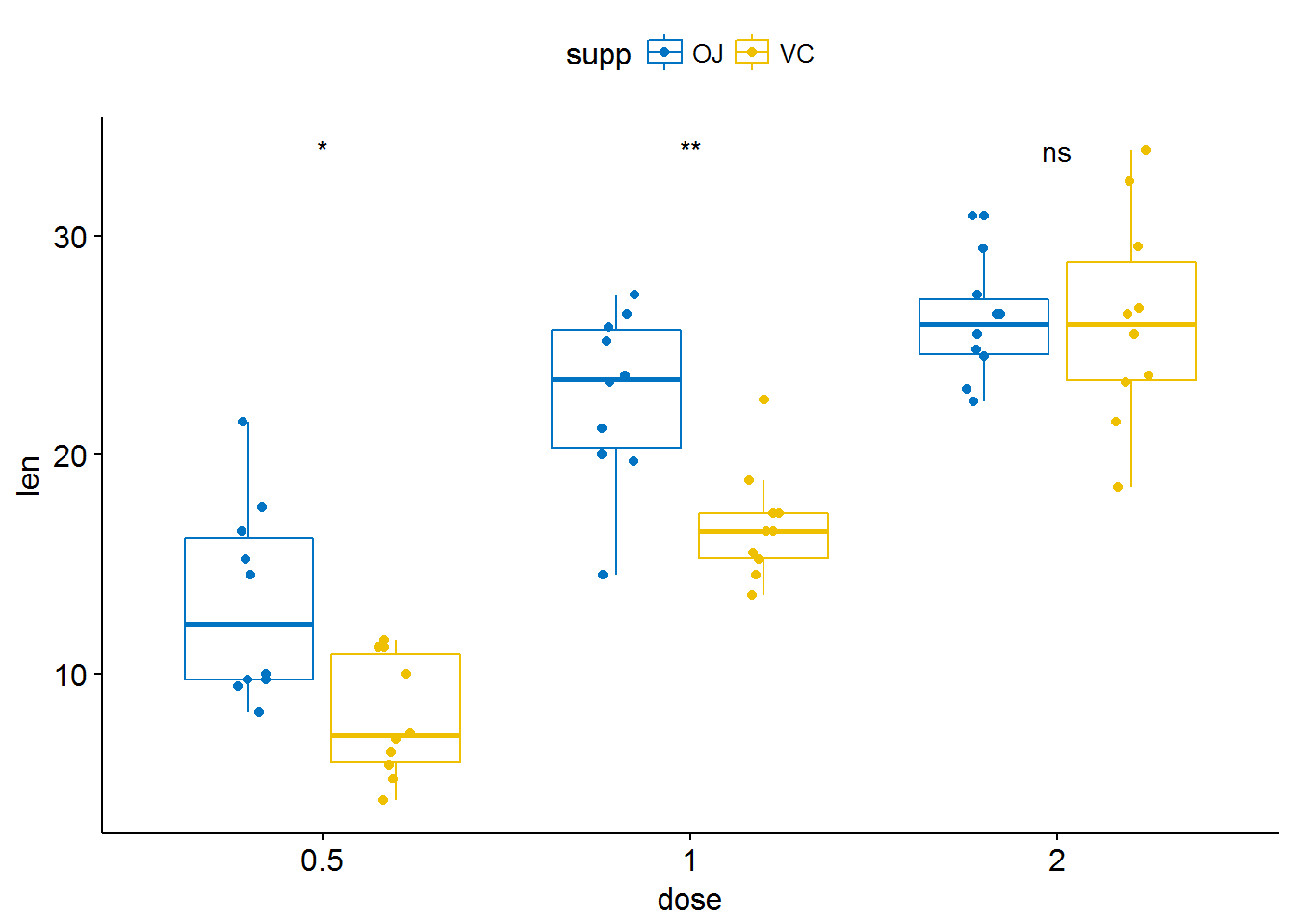
#label绘制显著性水平
p+stat_compare_means(label = "p.signif", label.x = 1.5)
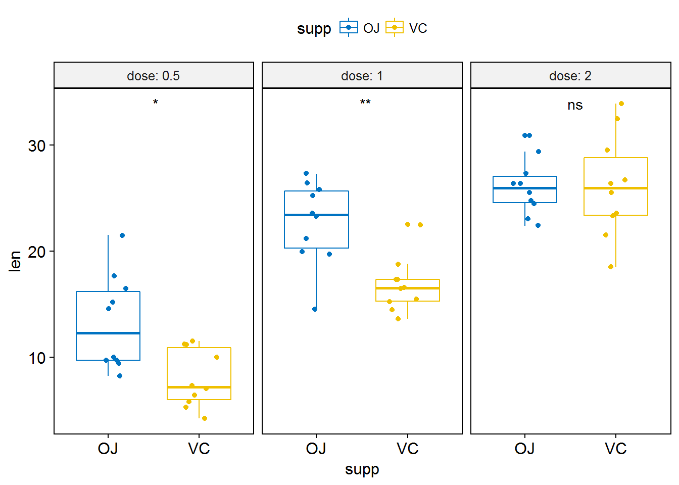
#将所有箱线图绘制在一个panel中
p <- ggboxplot(ToothGrowth, x="dose", y="len", color = "supp",
palette = "jco", add = "jitter")
p+stat_compare_means(aes(group=supp))
#只显示p-value
p+stat_compare_means(aes(group=supp), label = "p.format")
#显示显著性水平
p+stat_compare_means(aes(group=supp), label = "p.signif")
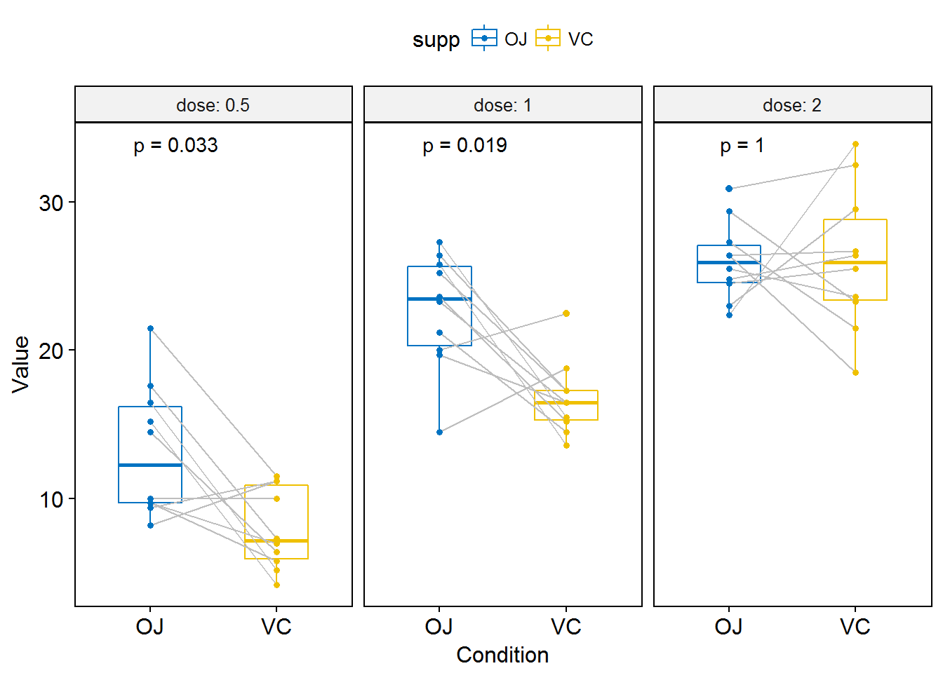
进行paired sample检验
compare_means(len~supp, data=ToothGrowth, group.by = "dose", paired = TRUE)
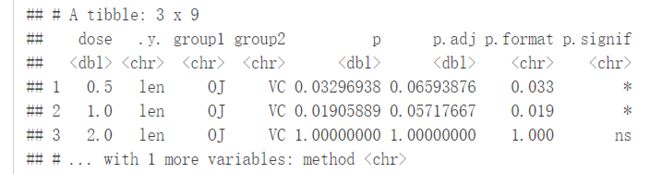
#可视化
p <- ggpaired(ToothGrowth, x="supp", y="len", color = "supp",
palette = "jco", line.color="gray", line.size=0.4, facet.by = "dose",
short.panel.labs = FALSE)#按dose分面
#只显示p-value
p+stat_compare_means(label = "p.format", paired = TRUE)
其他图形
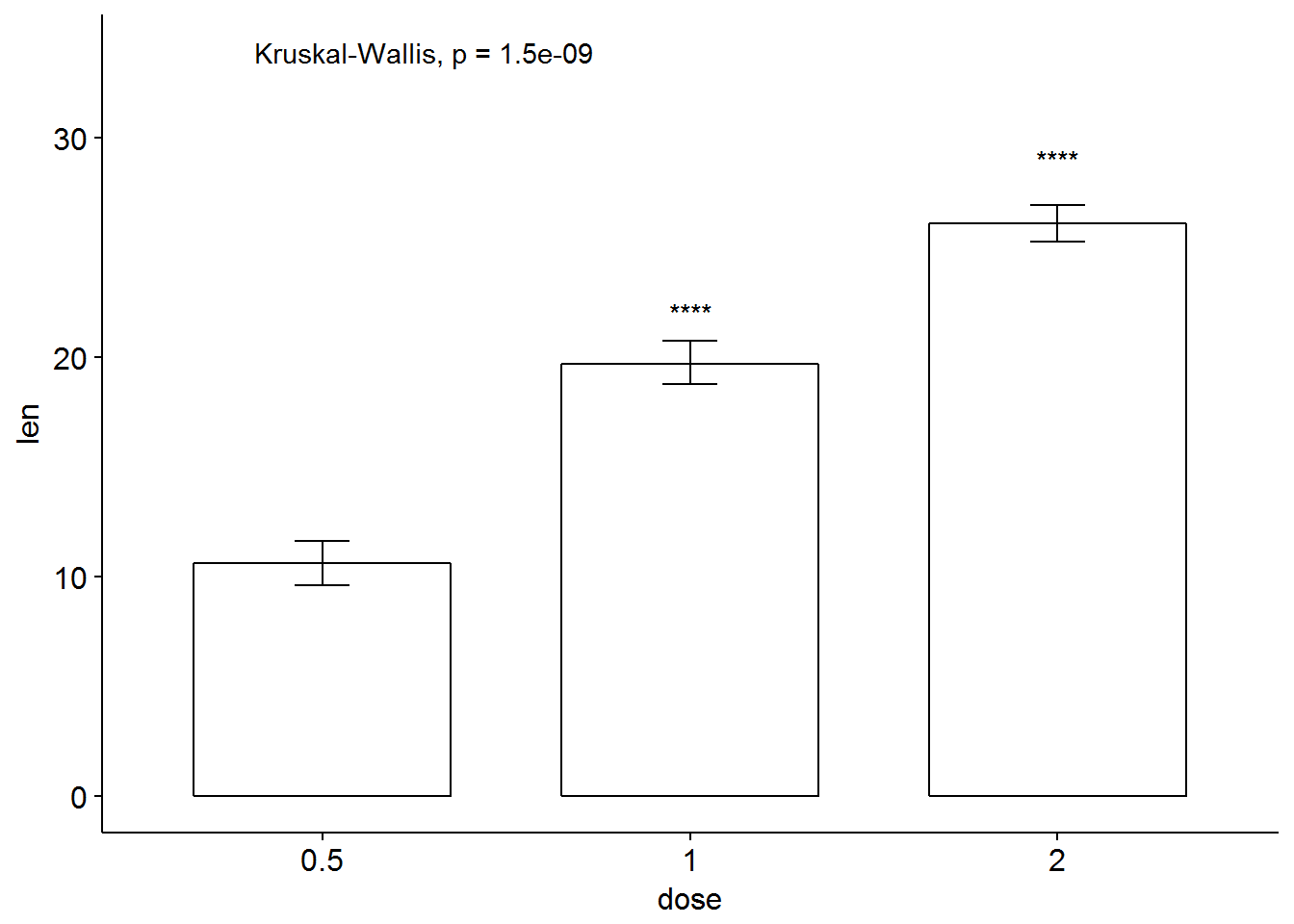
条形图与线图(一个分组变量)
#有误差棒的条形图,实际上我以前的文章里有纯粹用ggplot2实现
ggbarplot(ToothGrowth, x="dose", y="len", add = "mean_se")+
stat_compare_means()+
stat_compare_means(ref.group = "0.5", label = "p.signif", label.y = c(22, 29))
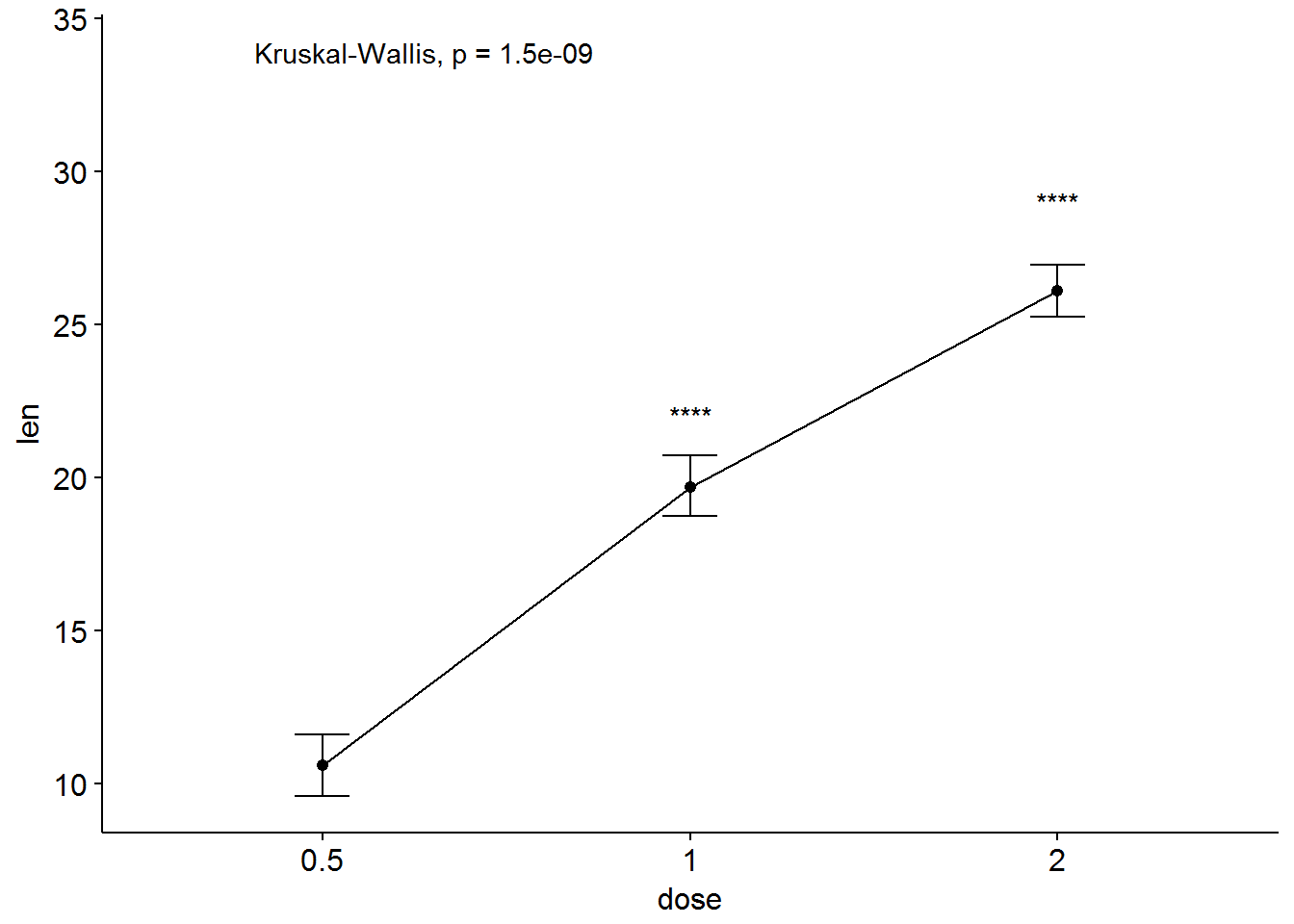
#有误差棒的线图
ggline(ToothGrowth, x="dose", y="len", add = "mean_se")+
stat_compare_means()+
stat_compare_means(ref.group = "0.5", label = "p.signif", label.y = c(22, 29))
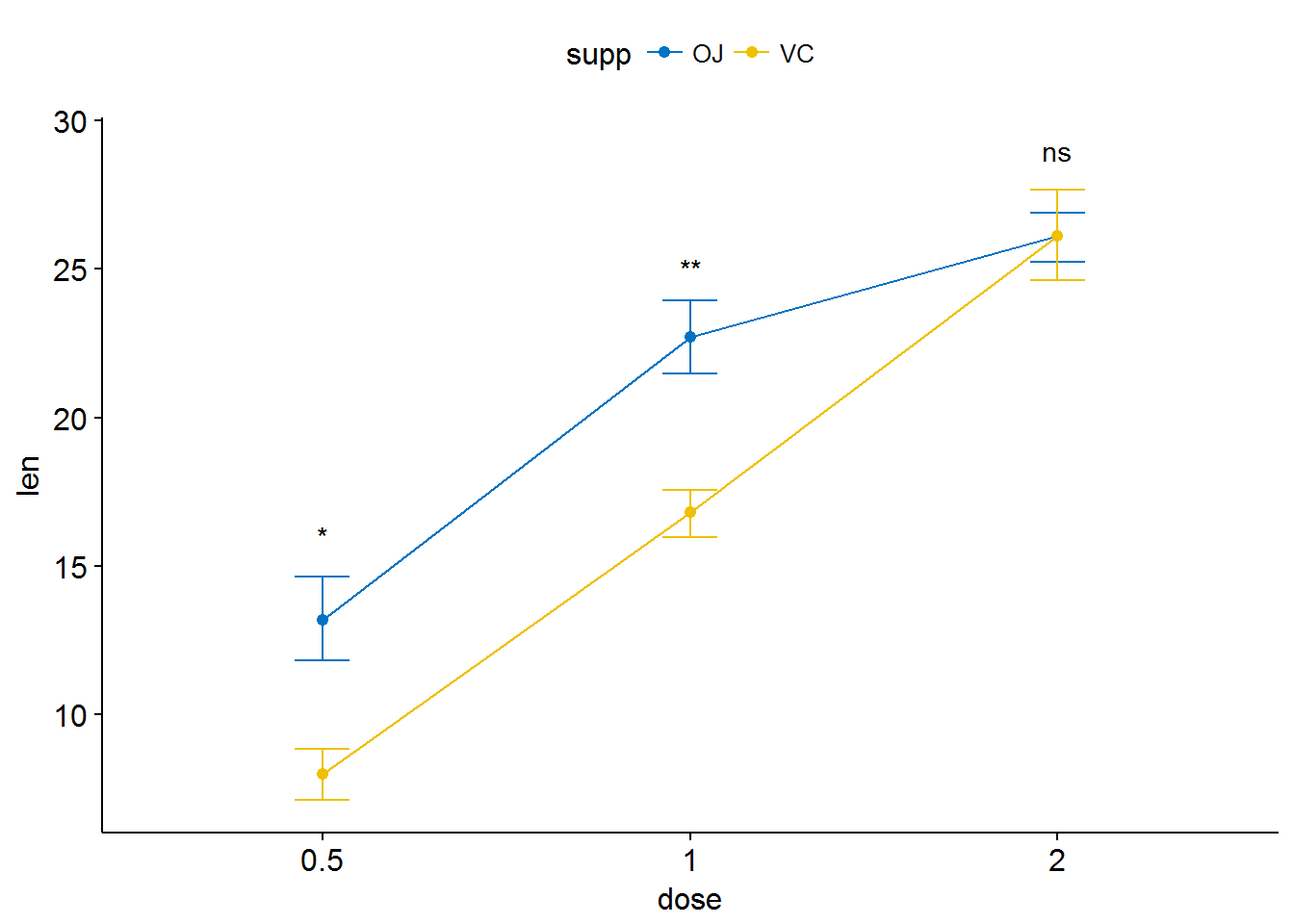
条形图与线图(两个分组变量)
ggbarplot(ToothGrowth, x="dose", y="len", add = "mean_se", color = "supp",
palette = "jco", position = position_dodge(0.8))+
stat_compare_means(aes(group=supp), label = "p.signif", label.y = 29)

ggline(ToothGrowth, x="dose", y="len", add = "mean_se", color = "supp",
palette = "jco")+
stat_compare_means(aes(group=supp), label = "p.signif", label.y = c(16, 25, 29))
Sessioninfo
sessionInfo()
## R version 3.4.0 (2017-04-21)
## Platform: x86_64-w64-mingw32/x64 (64-bit)
## Running under: Windows 8.1 x64 (build 9600)
##
## Matrix products: default
##
## locale:
## [1] LC_COLLATE=Chinese (Simplified)_China.936
## [2] LC_CTYPE=Chinese (Simplified)_China.936
## [3] LC_MONETARY=Chinese (Simplified)_China.936
## [4] LC_NUMERIC=C
## [5] LC_TIME=Chinese (Simplified)_China.936
##
## attached base packages:
## [1] stats graphics grDevices utils datasets methods base
##
## other attached packages:
## [1] survminer_0.4.0 ggpubr_0.1.3 magrittr_1.5 ggplot2_2.2.1
##
## loaded via a namespace (and not attached):
## [1] Rcpp_0.12.11 compiler_3.4.0 plyr_1.8.4
## [4] tools_3.4.0 digest_0.6.12 evaluate_0.10
## [7] tibble_1.3.3 gtable_0.2.0 nlme_3.1-131
## [10] lattice_0.20-35 rlang_0.1.1 Matrix_1.2-10
## [13] psych_1.7.5 ggsci_2.4 DBI_0.6-1
## [16] cmprsk_2.2-7 yaml_2.1.14 parallel_3.4.0
## [19] gridExtra_2.2.1 dplyr_0.5.0 stringr_1.2.0
## [22] knitr_1.16 survMisc_0.5.4 rprojroot_1.2
## [25] grid_3.4.0 data.table_1.10.4 KMsurv_0.1-5
## [28] R6_2.2.1 km.ci_0.5-2 survival_2.41-3
## [31] foreign_0.8-68 rmarkdown_1.5 reshape2_1.4.2
## [34] tidyr_0.6.3 purrr_0.2.2.2 splines_3.4.0
## [37] backports_1.1.0 scales_0.4.1 htmltools_0.3.6
## [40] assertthat_0.2.0 mnormt_1.5-5 xtable_1.8-2
## [43] colorspace_1.3-2 ggsignif_0.2.0 labeling_0.3
## [46] stringi_1.1.5 lazyeval_0.2.0 munsell_0.4.3
## [49] broom_0.4.2 zoo_1.8-0