第八章 模型篇:transfer learning for computer vision
参考教程:
transfer-learning
transfer-learning tutorial
文章目录
- transfer learning
-
- 对卷积网络进行finetune
- 把卷积网络作为特征提取器
- 何时、如何进行fine tune
- 代码示例
-
- 加载数据集
- 构建模型
-
- fine-tune 模型
- 模型作为feature extractor
- 定义train_loop和test_loop
- 定义超参数,开始训练
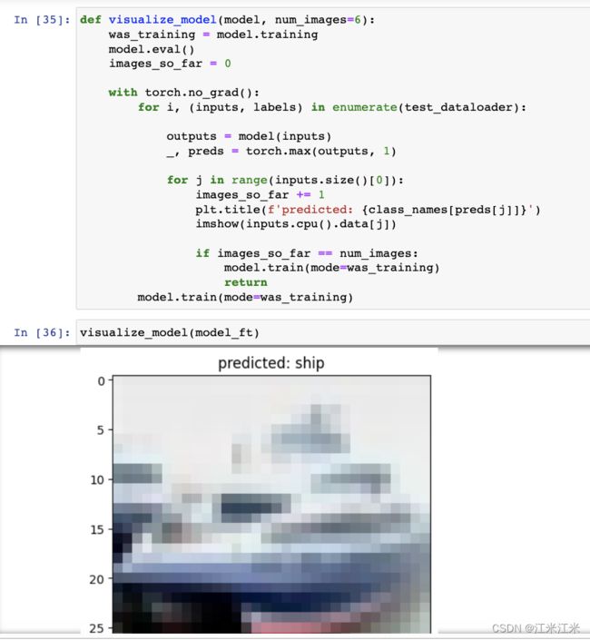
- 结果可视化
transfer learning
很少会有人从头开始训练一个卷积神经网络,因为并不是所有人都有机会接触到大量的数据。常用的选择是在一个非常大的模型上预训练一个模型,然后用这个模型为基础,或者固定它的参数用作特征提取,来完成特定的任务。
对卷积网络进行finetune
进行transfer-learning的一个方法是在基于大数据训练的模型上进行fine-tune。可以选择对模型的每一个层都进行fine-tune,也可以选择freeze特定的层(一般是比较浅的层)而只对模型的较深的层进行fine-tune。理论支持是,模型的浅层通常是一些通用的特征,比如edge或者colo blob,这些特征可以应用于多种类型的任务,而高层的特征则会更倾向于用于训练的原始数据集中的数据特点,因为不太能泛化到新数据上去。
把卷积网络作为特征提取器
将ConvNet作为一个特征提取器,通常是去掉它最后一个用于分类的全连接层,把剩余的层用来提取新数据的特征。你可以在该特征提取器后加上你自己的head,比如分类head或者回归head,用于完成你自己的任务。
何时、如何进行fine tune
使用哪种方法有多种因素决定,最主要的因素是你的新数据集的大小和它与原始数据集的相似度。
- 当你的新数据集很小,并和原始数据集比较相似时。
因为你的数据集很小,所以从过拟合的角度出发,不推荐在卷积网络上进行fine-tune。又因为你的数据和原始数据比较相似,所以卷积网络提取的高层特征和你的数据也是相关的。因此你可以直接卷积网络当作特征提取器,在此基础上训练一个线性分类器。 - 当你的新数据集很大,并和原始数据集比较相似时。
新数据集很大时,我们可以对整个网络进行fine-tune,因为我们不太会有过拟合的风险。 - 当你的新数据集很小,并和原始数据集不太相似时。
因为你的数据集很小,我们还是推荐只训练一个线性的分类器。但是新数据和原始数据又不相似,所以不建议在网络顶端接上新的分类器,因为网络顶端包含很多的dataset-specific的特征,所以更推荐的是从浅层网络的一个位置出发接上一个分类器。 - 当你的新数据集很大,并和原始数据集不太相似时。
因为你的数据集很大,我们仍然选择对整个网络进行fine-tune。因为通常情况下以一个pretrained-model对模型进行初始化的效果比随机初始化要好。
代码示例
我们使用与第四章 模型篇:模型训练与示例一样的流程进行模型训练。
加载数据集
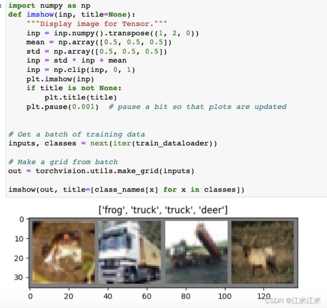
首先是加载数据集,方便起见我们直接使用torchvision中的cifar10数据进行训练。
transform = transforms.Compose(
    [transforms.ToTensor(),
     transforms.Normalize((0.5, 0.5, 0.5), (0.5, 0.5, 0.5))])

training_data = datasets.CIFAR10(
    root="data",
    train=True,
    download=True,
    transform=transform
)


test_data = datasets.CIFAR10(root='./data', train=False,
                                       download=True, transform=transform)

train_dataloader = DataLoader(training_data, batch_size = 64)
test_dataloader = DataLoader(test_data, batch_size = 64)
使用官方提供的代码对我们的dataset进行可视化,注意训练时使用的batchsize为64,这里可视化时为了方便暂时使用了batchsize=4。
构建模型
在第四章中我们用了自定义的model。在这里我们使用预训练好的模型,并对模型结构进行修改。
transfer-learning对模型的处理有两种,一种是fine-tune整个模型,一种是将模型作为feature-extractor。第二种和第一种的区别是,模型中的部分层被freeze,不在训练过程中更新。
fine-tune 模型
model_ft = models.resnet18(weights = 'IMAGENET1K_V1')
num_ftrs = model_ft.fc.in_features
model_ft.fc = nn.Linear(num_ftrs, 10) # 因为cifar10是十分类,所以输出这里为10
模型作为feature extractor
model_conv = torchvision.models.resnet18(weights='IMAGENET1K_V1')
for param in model_conv.parameters():
    param.requires_grad = False  # requires_grad 设为False,不随训练更新

# Parameters of newly constructed modules have requires_grad=True by default
num_ftrs = model_conv.fc.in_features
model_conv.fc = nn.Linear(num_ftrs, 10)
定义train_loop和test_loop
这两个部分直接参考第四章的代码就可以,复制过来直接使用。
# 训练过程的每个epoch的操作,代码来自pytorch_tutorial
def train_loop(dataloader, model, loss_fn, optimizer):
    size = len(dataloader.dataset)
    # Set the model to training mode - important for batch normalization and dropout layers
    # Unnecessary in this situation but added for best practices
    model.train()
    for batch, (X, y) in enumerate(dataloader):
        optimizer.zero_grad() # 重置梯度计算
        # Compute prediction and loss
        pred = model(X)
        loss = loss_fn(pred, y)

        # Backpropagation
        loss.backward() # 反向传播计算梯度
        optimizer.step() # 调整模型参数


        if batch % 10 == 0:
            loss, current = loss.item(), (batch + 1) * len(X)
            print(f"loss: {loss:>7f}  [{current:>5d}/{size:>5d}]")


def test_loop(dataloader, model, loss_fn):
    # Set the model to evaluation mode - important for batch normalization and dropout layers
    # Unnecessary in this situation but added for best practices
    model.eval()
    size = len(dataloader.dataset)
    num_batches = len(dataloader)
    test_loss, correct = 0, 0

    # Evaluating the model with torch.no_grad() ensures that no gradients are computed during test mode
    # also serves to reduce unnecessary gradient computations and memory usage for tensors with requires_grad=True
    with torch.no_grad():
        for X, y in dataloader:
            pred = model(X)
            test_loss += loss_fn(pred, y).item()
            correct += (pred.argmax(1) == y).type(torch.float).sum().item()

    test_loss /= num_batches
    correct /= size
    print(f"Test Error: \n Accuracy: {(100*correct):>0.1f}%, Avg loss: {test_loss:>8f} \n")
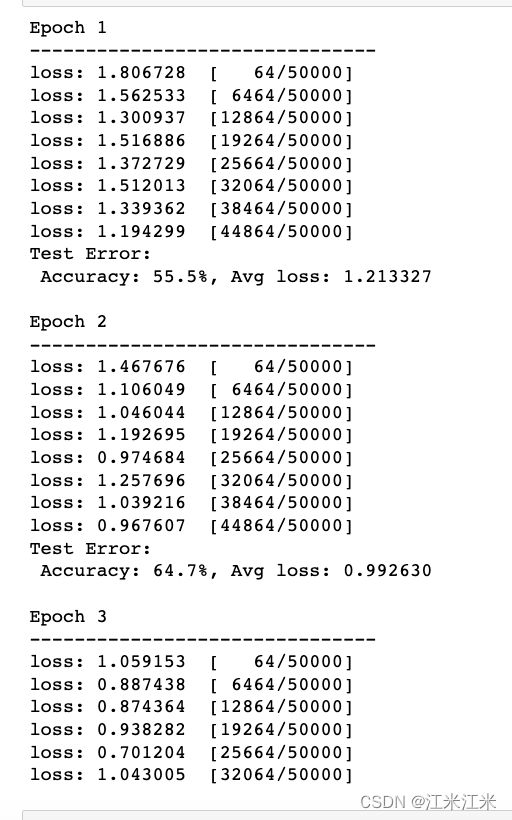
定义超参数,开始训练
全都准备好以后,我们定义一下要使用的优化器和loss,和一些别的超参数,就可以开始训练了。
learning_rate = 1e-3
momentum=0.9
epochs = 20

loss_fn = nn.CrossEntropyLoss()
optimizer = torch.optim.SGD(model.parameters(), lr=learning_rate,momentum=momentum)

for t in range(epochs):
    print(f"Epoch {t+1}\n-------------------------------")
    train_loop(train_dataloader, model_ft, loss_fn, optimizer)
    test_loop(test_dataloader, model_ft, loss_fn)
print("Done!")
因为是在个人pc跑的,所以就随便放一个效果。。。。。
结果可视化