【基于矢量射线的衍射积分 （VRBDI）】基于矢量射线的衍射积分 （VRBDI） 和仿真工具（Matlab代码实现）

欢迎来到本博客❤️❤️

博主优势：博客内容尽量做到思维缜密，逻辑清晰，为了方便读者。

⛳️座右铭：行百里者，半于九十。

本文目录如下：

目录

1 概述

2 运行结果

3 参考文献

4 Matlab代码实现及详细文章讲解

---

1 概述

• 基于矢量射线的衍射积分（Vector Ray-Based Diffraction Integral，VRBDI）是一种用于模拟光的衍射现象的方法。它基于矢量射线追踪技术，通过对光波的传播路径进行追踪和积分，来计算衍射图样。VRBDI方法可以用于模拟各种衍射现象，包括光栅衍射、衍射光栅、衍射孔径等。

  VRBDI方法的基本思想是将光波看作是由许多矢量射线组成的，每条射线具有位置、方向和振幅等属性。通过追踪这些射线的传播路径，并根据衍射积分的原理进行积分计算，可以得到衍射图样的近似解。VRBDI方法可以考虑光的波动性和干涉效应，适用于模拟复杂的衍射现象。

  在VRBDI方法的实现中，通常需要借助计算机仿真工具来进行数值计算和模拟。一些常用的仿真工具包括：

  1. MATLAB：MATLAB是一种常用的科学计算和仿真工具，它提供了丰富的数值计算和图形绘制函数，可以用于实现VRBDI方法的数值计算和模拟。

  2. Zemax：Zemax是一种专业的光学设计和仿真软件，它提供了强大的光学建模和分析功能，包括衍射现象的模拟和分析。可以使用Zemax来实现VRBDI方法的仿真。

  3. VirtualLab：VirtualLab是一种专业的光学仿真软件，它提供了全面的光学建模和仿真功能，包括衍射、干涉、衍射光栅等现象的模拟和分析。可以使用VirtualLab来实现VRBDI方法的仿真。

  这些仿真工具都具有强大的功能和灵活的使用方式，可以根据具体的需求选择合适的工具进行VRBDI方法的实现和仿真。

• 详细文章讲解见第4部分。

2 运行结果

 

 

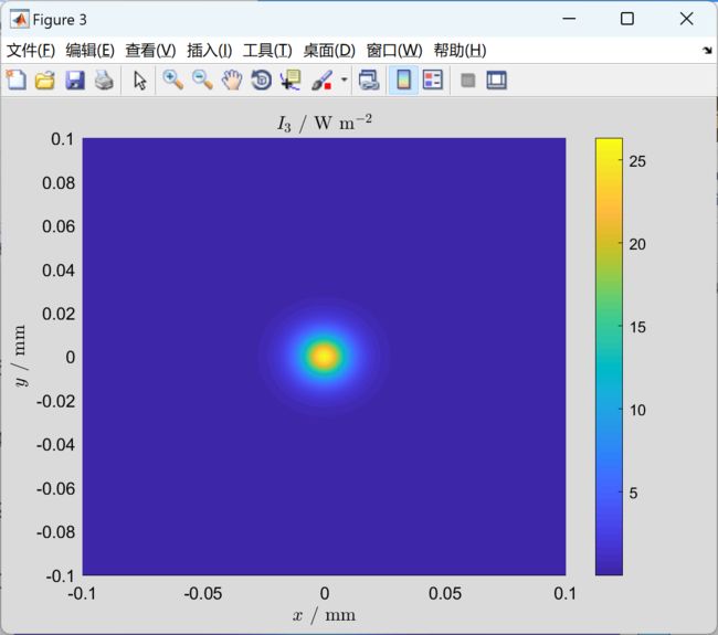
本文一共分为五个部分，这里仅展现第一部分结果图。

 部分代码：

%Definitions (all lengths in mm, wavelength in nm)

lambda=532;     %Wavelength
w0=2.3;         %Gaussian waist radius
zw=-10000;      %Distance from waist (negative value => beam convergent)
z0=10;          %Distance from input plane to front lens apex
z1=1;           %Distance from rear lens apex to intermediary plane
n=Sellmeier(lambda,'AIR');  %Refractive index immersion medium

b1=15;          %Edge length of square-shaped input window
b2=15;          %Edge length of square-shaped intermediary window
b3=0.2;         %Edge length of square-shaped output window
Pix1=55;        %Pixels along one dimension of input window
Pix2=99;        %Pixels along one dimension of intermediary and output 
                %window

%Lens parameters THORLABS LBF254-050-A ####################################

RL1=30.06;      %Front curvature radius
RL2=-172;       %Back curvature radius
TL=6.5;         %Center thickness
fB=46.4;        %Back focal distance
ApL=12.7;       %Aperture radius
nL=Sellmeier(lambda,'N-BK7');

%Remaining distance after lens to focal region

z2=fB-z1;

%Definition of lens component and initialization of System ################

SL=AddSurf([0 0 0],RL1,ApL,n,nL,-1,1);      %Initialization surface list SL
SL=AddSurf([0 0 TL],RL2,ApL,nL,n,-1,1,SL);  %Appending surface to SL    
Lens=DefComp([0 0 z0],[0 0 0],SL);          %Definition of Lens
System=AddComp(Lens);                       %Initialization of System with
                                            %Lens

%Definition of detector component and addition to System ################## 

SL=AddDet([0 0 0],1e30,1e30,n,0);           %Detector size should be large
Det=DefComp([0 0 z0+TL+z1],[0 0 0],SL);     %to catch all remaining rays!
System=AddComp(Det,System);                 %Appending Detector to System

%Definition of spatial point grids ########################################

[X1,Y1]=meshgrid(-b1/2:b1/(Pix1-1):b1/2);
[X2,Y2]=meshgrid(-b2/2:b2/(Pix2-1):b2/2);
[X3,Y3]=meshgrid(-b3/2:b3/(Pix2-1):b3/2);

%Reshaping of input and output grids for VDI propagation ##################

P2=[X2(:) Y2(:) 0*X2(:)];
P3=[X3(:) Y3(:) 0*X3(:)+z2];

%Definition of tangent electric field components on input plane ###########

E1x=GaussianField(w0,zw,lambda,n,b1,Pix1);
E1y=zeros(Pix1);

%Get irradiance and other field components on input plane #################

[I1,E1z,H1x,H1y,H1z]=GetIrrad(E1x,E1y,lambda,n,b1,b1);

%Get plane wave spectrum from input field ################################

3 参考文献

部分理论来源于网络，如有侵权请联系删除。

[1] B. Andreas, G. Mana, and C. Palmisano, "Vectorial ray-based diffraction integral," J. Opt. Soc. Am. A 32, 1403-1424 (2015).

[2]陈光炜, 陈光炜. 光学与光谱学实验指导[M]. 科学出版社, 2015.

[3]李大鹏, 李大鹏. 光学实验指导[M]. 高等教育出版社, 2017.

4 Matlab代码实现及详细文章讲解