书接上文——DETR评估可视化

在上一篇文章中，详细记录了如何使用官方开源的DETR项目开发训练自己的数据集，有详细的教程，感兴趣可以看下：
《DETR (DEtection TRansformer)基于自建数据集开发构建目标检测模型超详细教程》

在文末我还附上了自己简单的绘图实践，因为没有仔细研究过DETR项目，所以也就没有发现官方的项目中其实也是有对应的评估可视化实现的，如下所示：

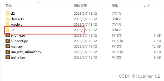
 对应模块如下所示：

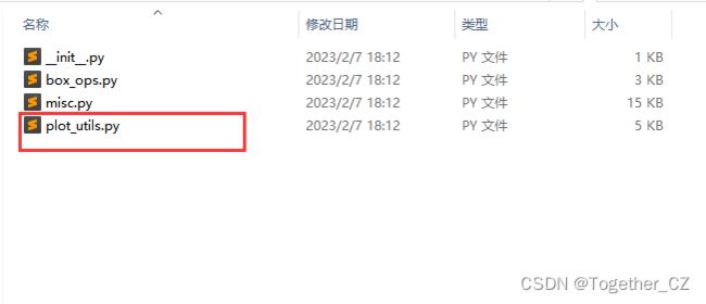
 接下来我们看下绘图模块的源码如下所示：

"""
Plotting utilities to visualize training logs.
"""
import torch
import pandas as pd
import numpy as np
import seaborn as sns
import matplotlib.pyplot as plt

from pathlib import Path, PurePath


def plot_logs(logs, fields=('class_error', 'loss_bbox_unscaled', 'mAP'), ewm_col=0, log_name='log.txt'):
    '''
    Function to plot specific fields from training log(s). Plots both training and test results.

    :: Inputs - logs = list containing Path objects, each pointing to individual dir with a log file
              - fields = which results to plot from each log file - plots both training and test for each field.
              - ewm_col = optional, which column to use as the exponential weighted smoothing of the plots
              - log_name = optional, name of log file if different than default 'log.txt'.

    :: Outputs - matplotlib plots of results in fields, color coded for each log file.
               - solid lines are training results, dashed lines are test results.

    '''
    func_name = "plot_utils.py::plot_logs"

    # verify logs is a list of Paths (list[Paths]) or single Pathlib object Path,
    # convert single Path to list to avoid 'not iterable' error

    if not isinstance(logs, list):
        if isinstance(logs, PurePath):
            logs = [logs]
            print(f"{func_name} info: logs param expects a list argument, converted to list[Path].")
        else:
            raise ValueError(f"{func_name} - invalid argument for logs parameter.\n \
            Expect list[Path] or single Path obj, received {type(logs)}")

    # Quality checks - verify valid dir(s), that every item in list is Path object, and that log_name exists in each dir
    for i, dir in enumerate(logs):
        if not isinstance(dir, PurePath):
            raise ValueError(f"{func_name} - non-Path object in logs argument of {type(dir)}: \n{dir}")
        if not dir.exists():
            raise ValueError(f"{func_name} - invalid directory in logs argument:\n{dir}")
        # verify log_name exists
        fn = Path(dir / log_name)
        if not fn.exists():
            print(f"-> missing {log_name}.  Have you gotten to Epoch 1 in training?")
            print(f"--> full path of missing log file: {fn}")
            return

    # load log file(s) and plot
    dfs = [pd.read_json(Path(p) / log_name, lines=True) for p in logs]

    fig, axs = plt.subplots(ncols=len(fields), figsize=(16, 5))

    for df, color in zip(dfs, sns.color_palette(n_colors=len(logs))):
        for j, field in enumerate(fields):
            if field == 'mAP':
                coco_eval = pd.DataFrame(
                    np.stack(df.test_coco_eval_bbox.dropna().values)[:, 1]
                ).ewm(com=ewm_col).mean()
                axs[j].plot(coco_eval, c=color)
            else:
                df.interpolate().ewm(com=ewm_col).mean().plot(
                    y=[f'train_{field}', f'test_{field}'],
                    ax=axs[j],
                    color=[color] * 2,
                    style=['-', '--']
                )
    for ax, field in zip(axs, fields):
        ax.legend([Path(p).name for p in logs])
        ax.set_title(field)


def plot_precision_recall(files, naming_scheme='iter'):
    if naming_scheme == 'exp_id':
        # name becomes exp_id
        names = [f.parts[-3] for f in files]
    elif naming_scheme == 'iter':
        names = [f.stem for f in files]
    else:
        raise ValueError(f'not supported {naming_scheme}')
    fig, axs = plt.subplots(ncols=2, figsize=(16, 5))
    for f, color, name in zip(files, sns.color_palette("Blues", n_colors=len(files)), names):
        data = torch.load(f)
        # precision is n_iou, n_points, n_cat, n_area, max_det
        precision = data['precision']
        recall = data['params'].recThrs
        scores = data['scores']
        # take precision for all classes, all areas and 100 detections
        precision = precision[0, :, :, 0, -1].mean(1)
        scores = scores[0, :, :, 0, -1].mean(1)
        prec = precision.mean()
        rec = data['recall'][0, :, 0, -1].mean()
        print(f'{naming_scheme} {name}: mAP@50={prec * 100: 05.1f}, ' +
              f'score={scores.mean():0.3f}, ' +
              f'f1={2 * prec * rec / (prec + rec + 1e-8):0.3f}'
              )
        axs[0].plot(recall, precision, c=color)
        axs[1].plot(recall, scores, c=color)

    axs[0].set_title('Precision / Recall')
    axs[0].legend(names)
    axs[1].set_title('Scores / Recall')
    axs[1].legend(names)
    return fig, axs

可以很清晰地看到：官方这里主要提供了两组绘图函数，分别是plot_logs对训练日志数据进行可视化的以及plot_precision_recall绘制模型精确率和召回率的函数。

接下来我们就以昨天模型开发的结果为基准来绘图，结果如下所示：

【日志数据可视化】

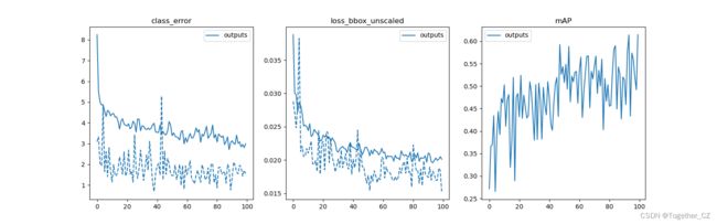
 跟我的想法差不多，主要就是选取了：训练-测试的loss、error以及mAP进行了可视化。

【精确率-召回率可视化】

 整体感觉比较“朴素”吧，跟YOLO系列的分割还是相差甚远的。

这里其实也可以加入一个F1值的可视化，因为F1是可以基于precision和recall计算得到的，这个感兴趣的话可以自行尝试一下。

接下来是推理，原生的推理效果图如下所示：

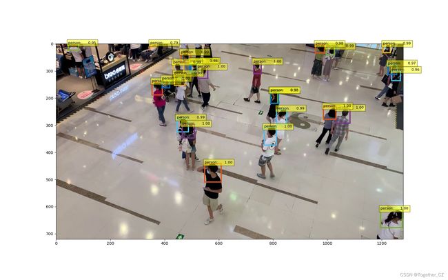
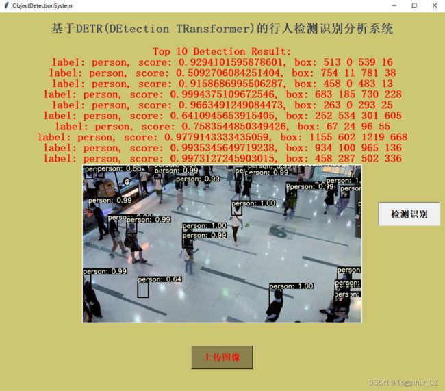
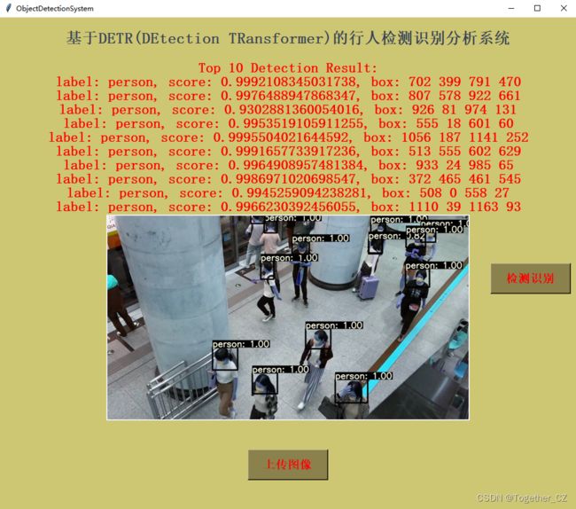
 感觉着实是不够美观，我结合了YOLO系列的推理可视化方法进行了融合改造，实例效果图如下所示：

 为了方便使用这个项目，开发了专用的可视化系统界面，实例推理效果如下所示：