斯坦福数据挖掘教程·第三版》读书笔记（英文版）Chapter 13 Neural Nets and Deep Learning

来源：《斯坦福数据挖掘教程·第三版》对应的公开英文书和PPT

Chapter 13 Neural Nets and Deep Learning

In this chapter, we shall consider the design of neural nets, which are collections of perceptrons, or nodes, where the outputs of one rank (or layer of nodes) becomes the inputs to nodes at the next layer. The last layer of nodes produces the outputs of the entire neural net. The training of neural nets with many layers requires enormous numbers of training examples, but has proven to be an extremely powerful technique, referred to as deep learning, when it can be used.

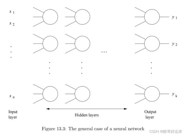
The general case is suggested by Fig. 13.3. The first, or input layer, is the input, which is presumed to be a vector of some length $n$. Each component of the vector $[x_1,x_2,...,x_n]$ is an input to the net. There are one or more hidden layers and finally, at the end, an output layer, which gives the result of the net. Each of the layers can have a different number of nodes, and in fact, choosing the right number of nodes at each layer is an important part of the design process for neural nets. Especially, note that the output layer can have many nodes. For instance, the neural net could classifyinputs into many different classes, with one output node for each class.

Each layer, except for the input layer, consists of one or more nodes, which we arrange in the column that represents that layer. We can think of each node as a perceptron. The inputs to a node are outputs of some or all of the nodes in the previous layer. So that we can assume the threshold for each node is zero, we can also allow a node to have an input that is a constant, typically 1. Associated with each input to each node is a weight. The output of the node depends on $\sum x_i{w}_i$, where the sum is over all the inputs $x_i$, and $w_i$ is the weight of that input. Sometimes, the output is either 0 or 1; the output is 1 if that sum is positive and 0 otherwise. However, it is often convenient, when trying to learn the weights for a neural net that solves some problem, to have outputs that are almost always close to 0 or 1, but may be slightly different. The reason, intuitively, is that it is then possible for the output of a node to be a continuous function of its inputs. We can then use gradient descent to converge to the ideal values of all the weights in the net.

Neural nets can differ in how the nodes at one layer are connected to nodes at the layer to its right. The most general case is when each node receives as inputs the outputs of every node of the previous layer. A layer that receives all outputs from the previous layer is said to be fully connected. Some other options for choosing interconnections are:

1. Random. For some m, we pick for each node m nodes from the previous layer and make those, and only those, be inputs to this node.
2. Pooled. Partition the nodes of one layer into some number of clusters. In the next layer, which is called a pooling layer, there is one node for each cluster, and this node has all and only the member of its cluster as inputs.
3. Convolutional. This approach to interconnection, which we discuss in more detail in the next section, views the nodes of each layer as arranged in a grid, typically two-dimensional. In a convolutional layer, a node corresponding to coordinates $(i,j)$ receive as inputs the nodes of the previous layer that have coordinates in some small region around $(i,j)$. For example, the node $(i,j)$ at one convolutional layer may have as inputs those nodes from the previous layer that correspond to coordinates $(p,q)$, where $i\le p\le i+2$ and $j\le q\le j+2$ (i.e., the square of side 3 whose lower-left corner is the point $(i,j)$.

Convolutional Neural Networks

A convolutional neural network, or CNN, contains one or more convolutional layers. There can also be non-convolutional layers, such as fully connected layers and pooled layers. However, there is an important additional constraint: the weights on the inputs must be the same for all nodes of a single convolutional layer. More precisely, suppose that each node $(i,j)$ in a convolutional layer receives $(i+u,j+v)$ as one of its inputs, where u and v are small constants.
Then there is a weight $w$ associated with $u$ and $v$ (but not with $i$ and $j$). For any $i$ and $j$, the weight on the input to the node for $(i,j)$ coming from the output of the node $i+u$, $j+v$) from the previous layer must be w. This restriction makes training a CNN much more efficient than training a general neural net. The reason is that there are many fewer parameters at each layer, and therefore, many fewer training examples can be used, than if each node or each layer has its own weights for the training process to discover.

Activation Functions

A node (perceptron) in a neural net is designed to give a 0 or 1 (yes or no) output. Often, we want to modify that output is one of several ways, so we apply an activation function to the output of a node. In some cases, the activation function takes all the outputs of a layer and modifies them as a group. the reason we need an activation function is as follows. The approach we shall use to learn good parameter values for the network is gradient descent. Thus, we need activation functions that “play well” with gradient descent. In particular, we look for activation functions with the following properties:

1. The function is continuous and differentiable everywhere (or almost everywhere).
2. The derivative of the function does not saturate (i.e., become very small, tending towards zero) over its expected input range. Very small derivatives tend to stall out the learning process.
3. The derivative does not explode (i.e., become very large, tending towards infinity), since this would lead to issues of numerical instability.

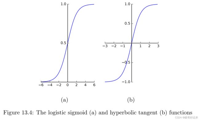
The Sigmoid

$$\sigma (x)=\frac{1}{1+e^{-x}}=\frac{e^x}{1+e^x}$$

The Hyperbolic Tangent

$$tanh(x)=\frac{e^x-e^{-x}}{e^x+e^{-x}}$$

Softmax

The softmax function differs from sigmoid functions in that it does not operate element-wise on a vector. Rather, the softmax function applies to an entire vector. If $x=[x_1,x_2,...,x_n]$, then its softmax $\mu (x)=[\mu (x_1),\mu (x_2),...,\mu (x_n)]$ where

$$\mu (x_i)=\frac{e^{x_i}}{{\sum }_j{e}^{x_i}}$$

Softmax pushes the largest component of the vector towards 1 while pushing all the other components towards zero. Also, all the outputs sum to 1, regardless of the sum of the components of the input vector. Thus, the output of the softmax function can be intepreted as a probability distribution.
A common application is to use softmax in the output layer for a classi-fication problem. The output vector has a component corresponding to each target class, and the softmax output is interpreted as the probability of the input belonging to the corresponding class.

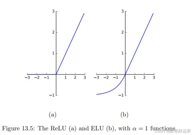
The rectified linear unit, or ReLU, is defined as:

In modern neural nets, a version of ReLU has replaced sigmoid as the default choice of activation function. The popularity of ReLU derives from two prerties:

1. The gradient of ReLU remains constant and never saturates for positive x, speeding up training. It has been found in practice that networks that use ReLU offer a significant speedup in training compared to sigmoid activation.
2. Both the function and its derivative can be computed using elementary and efficient mathematical operations (no exponentiation). ReLU does suffer from a problem related to the saturation of its derivative when $x<0$. Once a node’s input values become negative, it is possible that the node’s output get “stuck” at 0 through the rest of the training. This is called the dying ReLU problem.

The Leaky ReLU attempts to fix this problem by defining the activation function as follows:

where $\alpha$ is typically a small positive value such as 0.01. The Parametric ReLU (PReLU) makes $\alpha$ a parameter to be optimized as part of the learning process. An improvement on both the original and leaky ReLU functions is Exponential Linear Unit, or ELU. This function is defined as:

where $\alpha \ge 0$ is a hyperparameter. That is, α is held fixed during the learning process, but we can repeat the learning process with different values of α to find the best value for our problem. The node’s value saturates to $-\alpha$ for large negative values of $x$, and a typical choice is $\alpha =1$. ELU’s drive the mean activation of nodes towards zero, which appears to speed up the learning process compared to other ReLU variants.

One way to deal with this issue is to use the Huber Loss. Suppose $z=y-\hat{y}$, and δ is a constant. The Huber Loss $L_{\delta }$ is given by:

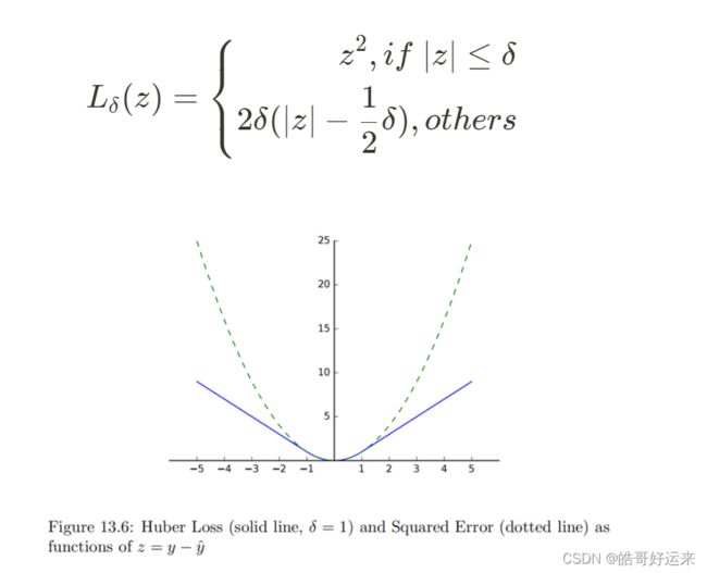
In the case where we have a vector y of outputs rather than a single output, we use $||y-\hat{y}||$ in place of $|y-\hat{y}|$ in the definitions of mean squared error and Huber loss.

That is, $H(p)$, the entropy of a discrete probability distribution p is:

$$H(p)=-\sum _{i=1}^n{p}_{i}log{p}_i$$

A well-known result from information theory states that the average number of bits in
this case is the cross entropy $H(p,q)$, defined as:

$$H(p,q)=-\sum _{i=1}^n{p}_{i}log{q}_i$$

Note that $H(p,p)=H(p)$, and in general $H(p,q)\ge H(p)$. The difference between the cross entropy and the entropy is the average number of additional bits needed per symbol. It is a reasonable measure of the distance between the distributions p and q, called the Kullblack-Liebler divergence (KL-divergence) and denoted $D(p||q)$:

$$D(p||q)=H(p,q)-H(p)=\sum _{i=1}^n{p}_{i}log\frac{p_i}{q_i}$$

Convolutional Neural Networks

Convolutional Layers

Convolutional layers make use of the fact that image features often are described by small contiguous areas in the image. For example, at the first convolutional layer, we might recognize small sections of edges in the image. At later layers, more complex structures, such as features that look like flower petals or eyes might be recognized. The idea that simplifies the calculation is the fact that the recognition of features such as edges does not depend on where in the image the edge is. Thus, we can train a single node to recognize a small section of edge, say an edge through a 5 × 5 region of pixels. This idea benefits us in two ways.

1. The node in question needs only inputs from 25 pixels corresponding to any 5 × 5 square, not inputs from all 224 × 224 pixels. That saves us a lot in the representation of the trained CNN.
2. The number of weights that we need to learn in the training process is greatly reduced. For each node in the layer, we require only one weight for each input to that node – say 75 weights if a pixel is represented by RGB values, not the 150,528 weights that we suggested above would be needed for an ordinary, fully connected layer.

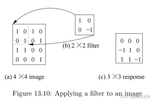
We shall think of the nodes in a convolutional layer as filters for learning features. A filter examines a small spatially contiguous area of the image – traditionally, a small square area such as a 5 × 5 square of pixels. Moreover, since many features of interest may occur anywhere in the input image (and possibly in more than one location), we apply the same filter at many locations on the input.
To keep things simple, suppose the input consists of monochromatic images, that is, grey-scale images whose pixels are each a single value. Each image is thus encoded by a 2-dimensional pixel array of size 224 × 224. A 5 × 5 filter F is encoded by a 5 × 5 weight matrix W and single bias parameter b. When the filter is applied on a similarly-sized square region of input image X with the top left corner of the filter aligned with the image pixel $x_{ij}$ , the response of the filter at this position, denoted $r_{ij}$ , is given by:

$$r_{ij}=\sum _{k=0}^4\sum _{l=0}^4{x}_{i+k,j+l}{w}_{kl}+b$$

When we deal with color images, the input has three channels. That is, each pixel is represented by three values, one for each color. Suppose we have a color image of size 224 × 224 × 3. The filter’s output will also have three channels, and so the filter is now encoded by a 5 × 5 × 3 weight matrix W and single bias parameter b. The activation map R still remains 5 × 5, with each response given by:

$$r_{ij}=\sum _{k=0}^4\sum _{l=0}^4\sum _{d=1}^3{x}_{i+k,j+l,d}{w}_{kld}+b$$

In our example, we imagined a filter of size 5. In general, the size of the filter is a hyperparameter of the convolutional layer. Filters of size 3, 4, or 5 are most commonly used. Note that the filter size specifies only the width and height of the filter; the number of channels of the filter always matches the number of channels of the input.

The activation map in our example is slightly smaller than the input. In many cases, it is convenient to have the activation map be of the same size as the input. We can expand the response by using zero padding: adding additional rows and columns of zeros to pad out the input. A zero padding of p corresponds to adding p rows of zeros each to the top and bottom, and p columns to the left and right, increasing the dimensionality of the input by 2p along both width and height. A zero padding of 2 in our example would augment the input size to 228 × 228 and result in an activation map of size 224 × 224, the same size as the original input image.

The third hyperparameter of interest is stride. In our example, we assumed that we apply the filter at every possible point in the input image. We could think instead of sliding the filter one pixel at a time along the width and height of the input, corresponding to a stride s = 1. Instead, we could slide the filter along the width and the height of image two or three pixels at a time, corresponding to a stride s of 2 or 3. The larger the stride, the smaller the activation map compared to the input.

Suppose the input is an $m\times m$ square of pixels, the output an $n\times n$ square, filter size is f, stride is s, and zero padding is p. It is easily seen that:

$$n=(m-f+2p)/s+1$$

The set of $k$ filters together constitute a convolutional layer. Given input with $d$ channels, a filter of size $f$ requires $d{f}^2+1$ parameters ($d{f}^2$ weight parameters and 1 bias parameter). Therefore, a convolutional layer of k such filters uses $k(d{f}^2+1)$ parameters.

A pooling layer takes as input the output of a convolutional layer and produces an output with smaller spatial extent. The size reduction is accomplished by using a pooling function to compute aggregates over small contiguous regions of the input. For example we might use max pooling over nonoverlapping $2\times 2$ regions of the input; in this case there is an output node corresponding to every nonoverlapping $2\times 2$ region of the input, with the output value being the maximum value among the 4 inputs in the region. The aggregation operates independently on each channel of the input. The resulting output layer is 25% the size of the input layer. There are three elements in defining a pooling layer:

1. The pooling function, which is most commonly the max function but could in theory be any aggregate function, such as average.
2. The size $f$ of each pool, which specifies that each pool uses an $f\times f$ square of inputs.
3. The stride $s$ between pools, analogous to the stride used in the convolutional layer.

Recurrent Neural Networks

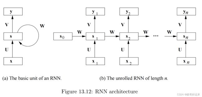
1. The RNN has inputs at all (or almost all) layers, and not just at the first layer.
2. The weights at each of the first n layers are constrained to be the same; these weights are the matrices U and W in Equation 13.5 below. Thus, each of the first n layers has the same set of nodes, and corresponding nodes from each of the layers share weights (and are thus really the same node), just as nodes of a CNN representing different locations share weights and are thus really the same node.

It is simplest to assume that our RNN’s inputs are fixed-length sequences of length $n$. In this case, we simply unroll the RNN to contain n time steps. In practice, many applications have to deal with variable-length sequences e.g., sentences of varying lengths. There are two approaches to deal with this situation:

1. Zero-padding. Fix n to be the longest sequence we process, and pad out shorter sequences to be length n.
2. Bucketing. Group sequences according to length, and build a separate RNN for each length.

Long Short-Term Memory (LSTM)

The LSTM model is a refinement of the basic RNN model to address the problem of learning long-distance associations. In the past few years, LSTM has become popular as the de-facto sequence-learning model, and has been used with success in many applications. Let us understand the intuition behind the LSTM model before we describe it formally. The main elements of the LSTM model are:

1. The ability to forget information by purging it from memory. For example, when analyzing a text we might want to discard information about a sentence when it ends. Or when analyzing a the sequence of frames in a movie, we might want to forget about the location of a scene when the next scene begins.
2. The ability to save selected information into memory. For example, when we process product reviews, we might want to save only words expressing opinions (e.g., excellent, terrible) and ignore other words.
3. The ability to focus only on the aspects of memory that are immediately relevant. For example, focus only on information about the characters of the current movie scene, or only on the subject of the sentence currently being analyzed. We can implement this focus by using a 2-tier architecture: a long-term memory that retains information about the entire processed prefix of the sequence, and a working memory that is restricted to the items of immediate relevance.

The RNN model has a single hidden state vector $s_t$ at time $t$. The LSTM model adds an additional state vector $c_t$, called the cell state, for each time $t$. Intuitively, the hidden state corresponds to working memory and the cell state corresponds to long-term memory. Both state vectors are of the same length, and both have entries in the range $[-1,1]$. We may imagine the working memory having most of its entries near zero with only the relevant entries turned “on.”

Dropout

Dropout is a technique that reduces overfitting by making random changes to the underlying deep neural network. Recall that when we train using stochastic gradient descent, at each step we sample at random a minibatch of inputs to process. When using dropout, we also select at random a certain fraction (say half) of all the hidden nodes from the network and delete them, along with any edges connected to them. We then perform forward propagation and backpropagation for the minibatch using this modified network, and update the weights and biases. After processing the minibatch, we restore all the deleted nodes and edges. When we sample the next minibatch, we delete a different random subset of nodes and repeat the training process.

The fraction of hidden nodes deleted each time is a hyperparameter called the dropout rate. When training is complete, and we actually use the full network, we need to take into account that the full network contains a larger number of hidden nodes than the networks used for training. We therefore need to scale the weight on each outgoing edge from a hidden node by the dropout rate.

Why does dropout reduce overfitting? Several hypotheses have been put forward, but perhaps the most convincing argument is that dropout allows a single neural network to behave effectively as a collection of neural networks. Imagine that we have a collection of neural networks, each with a different network topology. Suppose we trained each network independently using the training data, and used some kind of voting or averaging scheme to create a higher-level model. Such a scheme would perform better than any of the individual networks. The dropout technique simulates this setup without explicitly creating a collection of neural networks.

Summary of Chapter 13

• Neural Nets: A neural net is a collection of perceptrons (nodes), usually organized in layers, where the outputs from one layer provide inputs to the next layers. The first (inout) layer takes external inputs, and the last (output) layer indicates the class of the input. Other layers in the middle are called hidden layers and generally are trained to recognize intermediate concepts needed to determine the output.
• Types of Layers: Many layers are fully connected, meaning that each node in the layer has all the nodes of the previous layer as inputs. Other layers are pooled, meaning that the nodes of the previous layer are partitioned, and each node of this layer takes as input only the nodes of one block of the partition. Convolutional layers are also used, especially in image processing applications.
• Convolutional Layers: Convolutional layers can be viewed as if their nodes were organized into a two-dimensional array of pixels, with each pixel represented by the same collection of nodes. The weights on corresponding nodes from different pixels must be the same, so they are in effect the same node, and we need learn only one set of weights for each family of nodes, one from each pixel.
• Activation Functions: The output of a node in a neural net is determined by first taking the weighted sum of its inputs, using the weights that are learned during the process of training the net. An activation function is then applied to this sum. Common activation functions include the sigmoid function, the hyperbolic tangent, softmax, and various forms of linear recified unit functions.
• Loss Functions: These measure the difference between the output of the net and the correct output according to the training set. Commonly used loss functions include squared-error loss, Huber loss, classification loss, and cross-entropy loss.
• Training a Neural Net: We train a neural net by repeatedly computing the output of the net on training examples and computing the average loss on the training examples. Weights on the nodes are then adjusted by propagating the loss backward through the net, using the backpropagation algorithm.
• Backpropagation: By choosing our activation functions and loss functions to be differentiable, we can compute a deriative of the loss function with respect to every weight in the network. Thus, we can determine the direction in which to adjust each weight to reduce the loss. Using the chain rule, these directions can be computed layer-by-layer, from the output to the input.
• Convolutional Neural Networks: These typically consist of a large number of convolutional layers, along with pooled layers and fully connected layers. They are well suited to processing images, where the first convolutional layers recognize simple features, such as boundries, and later layers recognize progressively more complex features.
• Recurrent Neural Networks: These are designed to recognize sequences, such as sentences (sequences of words). There is one layer for each position in the sequence, and the nodes are divided into families, which each have one node at each layer. The nodes of a family are constrained to have the same weights, so the training process therefore needs to deal with a relatively small number of weights.
• Long Short-Term Memory Networks: These improve on RNN’s by adding a second state vector – the cell state – to enable some information about the sequence to be retained, while most information is forgotten after a while. In addition, we learn gate vectors that control what information is retained from the input, the state, and the output.
• Avoiding Overfitting: There are a number of specialized techniques designed to avoid overfitting a deep network. These include penalizing large weights, randomly dropping some nodes each time we apply a step of gradient descent, and use of a validation set to enable us to stop training when the loss on the validation set bottoms out.