机器学习笔记之优化算法(八)简单认识Wolfe Condition的收敛性证明

引言

上一节介绍了非精确搜索方法——$\text{Wolfe}$准则。本节将简单认识：$\text{Wolfe}$准则的收敛性证明。

回顾：$\text{Wolfe}$准则

关于先搜索方法表示如下：
$$x_{k+1}=x_k+{\alpha }_k\cdot {\mathcal{P}}_k$$
在数值解迭代过程中，当前时刻的迭代步长结果${\alpha }_k$未确定的情况下，将步长设为变量$\alpha$。在下降方向${\mathcal{P}}_k$确定的条件下，关于$x_{k+1}$的目标函数结果$f(x_{k+1})$可表示为关于变量$\alpha$的函数$\varphi (\alpha )$：
$$f(x_{k+1})=f(x_k+\alpha \cdot {\mathcal{P}}_k)=\varphi (\alpha )$$
由于$\{f(x_k){\}}_{k=0}^{\infty }$服从严格的单调性仅是目标函数收敛至最优解：$\{f(x_k){\}}_{k=0}^{\infty }\Rightarrow f^{\ast }$的必要不充分条件；因而需要相比更严格的条件使目标函数收敛至最优解：$\text{Armijo}$准则、$\text{Glodstein}$准则与$\text{Wolfe}$准则：
$$\begin{array}{rl}& \text{Armijo Condition : }\{\begin{array}{l}\varphi (\alpha )<f(x_k)+{\mathcal{C}}_1\cdot [\nabla f(x_k){]}^T{\mathcal{P}}_k\cdot \alpha \\ \\ {\mathcal{C}}_1\in (0,1)\end{array}\\ & \text{Glodstein Condition : }\{\begin{array}{l}f(x_k)+(1-\mathcal{C})\cdot [\nabla f(x_k){]}^T{\mathcal{P}}_k\cdot \alpha \le \varphi (\alpha )\le f(x_k)+\mathcal{C}\cdot [\nabla f(x_k){]}^T{\mathcal{P}}_k\cdot \alpha \\ \\ \mathcal{C}\in \begin{array}{r}\left(0,\frac{1}{2}\right)\end{array}\end{array}\end{array}$$

而$\text{Wolfe}$准则的初衷是为了处理$\text{Armijo}$准则与$\text{Goldstein}$准则的共同弊端：仅通过划分边界$(\text{Armijo})$或者划分边界构成的范围$(\text{Glodstein})$对相应的$\alpha$结果进行筛选，而被选择的$\alpha$结果是否存在意义$?$ 未知。

基于上述因素，$\text{Wlofe}$准则在$\text{Armijo}$准则的基础上，建立软性规则以筛选优质的$\alpha$结果：
其中$\begin{array}{r}{\varphi }^{\prime }(\alpha )=\frac{\partial f(x_k+\alpha \cdot {\mathcal{P}}_k)}{\partial \alpha }={\left[\nabla f(x_k+\alpha \cdot {\mathcal{P}}_k)\right]}^T{\mathcal{P}}_k\end{array}$。
$$\{\begin{array}{l}\varphi (\alpha )\le f(x_k)+{\mathcal{C}}_1\cdot [\nabla f(x_k){]}^T{\mathcal{P}}_k\cdot \alpha \\ {\varphi }^{\prime }(\alpha )\ge {\mathcal{C}}_2\cdot [\nabla f(x_k){]}^T{\mathcal{P}}_k\\ {\mathcal{C}}_1\in (0,1)\\ {\mathcal{C}}_2\in ({\mathcal{C}}_1,1)\end{array}$$
本节以$\text{Wolfe}$准则为例，简单介绍该准则的收敛性证明。

准备工作

推导条件介绍

• 关于目标函数优化的终极目标：$\underset{\mathcal{X}\in {\mathbb{R}}^n}{\min }f(\mathcal{X})$，因而对于目标函数$f(\mathcal{X})$，需要满足：向下有界，并且在定义域内连续可微；
  这属于函数自身的性质，在迭代过程中不能无限地小下去。

• 关于$f(\mathcal{X})$的梯度函数$\nabla f(\mathcal{X})$，需要在定义域内满足利普希茨连续$(\text{Lipschitz Continuity})$。对应数学符号表示如下：
  其中$\mathcal{L}$是一个常数。
  $$\forall x,\hat{x}\in {\mathbb{R}}^n,\exists \mathcal{L}:s.t.||\nabla f(x)-\nabla f(\hat{x})||\le \mathcal{L}\cdot ||x-\hat{x}||$$
  如果一个普通函数$\mathcal{G}(x)$满足利普希兹连续，可以将上述描述使用$\mathcal{G}(x)$进行替换，并进行简单变换：
  ∣ ∣ G ( x ) − G ( x ^ ) ∣ ∣ ≤ L ⋅ ∣ ∣ x − x ^ ∣ ∣ ⇒ ∣ ∣ G ( x ) − G ( x ^ ) x − x ^ ∣ ∣ ≤ L ||\mathcal G(x) - \mathcal G(\hat x)|| \leq \mathcal L \cdot ||x - \hat x|| \Rightarrow \left|\left|\frac{\mathcal G(x) - \mathcal G(\hat x)}{x - \hat x}\right|\right| \leq \mathcal L ∣∣G(x)−G(x^)∣∣≤L⋅∣∣x−x^∣∣⇒ ​ ​x−x^G(x)−G(x^)​ ​ ​≤L
  关于小于号左侧的式子格式： ∣ ∣ G ( x ) − G ( x ^ ) x − x ^ ∣ ∣ \begin{aligned}\left|\left|\frac{\mathcal G(x) - \mathcal G(\hat x)}{x - \hat x}\right|\right|\end{aligned} ​ ​x−x^G(x)−G(x^)​ ​ ​​，根据拉格朗日中值定理，可将该式表示为如下形式：
  ∃ ξ ∈ ( x , x ^ ) ⇒ ∣ ∣ G ( x ) − G ( x ^ ) x − x ^ ∣ ∣ = G ′ ( ξ ) \exist \xi \in (x,\hat x) \Rightarrow \begin{aligned}\left|\left|\frac{\mathcal G(x) - \mathcal G(\hat x)}{x - \hat x}\right|\right|\end{aligned} = \mathcal G'(\xi) ∃ξ∈(x,x^)⇒ ​ ​x−x^G(x)−G(x^)​ ​ ​​=G′(ξ)
  从而将利普希兹连续描述为如下形式：
  $$\exists \xi \in (x,\hat{x})\Rightarrow ||{\mathcal{G}}^{\prime }(\xi )||\le \mathcal{L}$$
  这意味着(不严谨)：关于函数$\mathcal{G}(x)$的一阶导函数${\mathcal{G}}^{\prime }(x)$存在上界$\mathcal{L}$。回到条件中，关于$\nabla f(\mathcal{X})$服从利普希兹连续可理解为：对目标函数的二阶梯度结果进行约束：
  $$\begin{array}{r}\frac{\partial \nabla f(\mathcal{X})}{\partial \mathcal{X}}\end{array}\le \mathcal{L}$$
  根据二阶梯度的几何意义，该条件本质上是对目标函数$f(\mathcal{X})$中斜率的变化量进行约束。关于不满足利普希兹连续的函数示例：$f(x)=x^2$。对应函数图像表示如下：
  
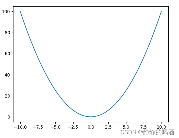
  关于该函数的一阶导函数$\begin{array}{r}\frac{\partial f}{\partial x}=2x\end{array}$，是一个关于$x$的一次函数，在定义域$x\in \mathbb{R}$中，其并不受某常数$\mathcal{L}$的约束。
  当$x\Rightarrow \infty$时，对应的$\begin{array}{r}\frac{\partial f}{\partial x}\Rightarrow \infty \end{array}$。
  再如：$\begin{array}{r}f(x)=\frac{1}{x}\end{array}$。对应函数图像表示如下：
  
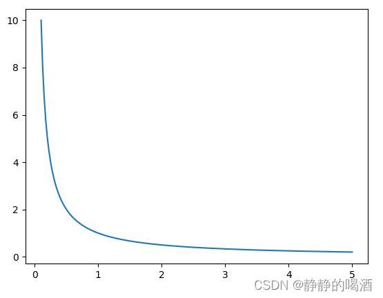
  同理，关于该函数的一阶导函数$\begin{array}{r}\frac{\partial f}{\partial x}=-\frac{1}{x^2}\end{array}$，在其定义域$x>0$中，其同样不受某常数$\mathcal{L}$的约束。
  当$x\Rightarrow 0$时，对应的$\begin{array}{r}\frac{\partial f}{\partial x}=-\infty \end{array}$。
  可以看出：上述两个例子在其对应的定义域内均是连续的，但它们不满足利普希兹连续。也就是说：利普希兹连续的条件更强。
  关于连续相关概念按照条件强度对比表示为：连续 $<$ 一致连续 $<$ 利普希兹连续(利普希兹条件)。

  • 上述条件强度可理解为：
    若某函数在其定义域内满足利普希兹连续，那么该函数一定满足一致连续和连续，反之不行；
    同理，若某函数在其定义域内满足一致连续，那么该函数一定满足连续，反之不行。
  • 其中一致连续与连续之间的区别可描述为：连续仅要求函数在其定义域内没有断点或者跳跃的情况;而一致连续在没有断点或者跳跃的基础上，还需要满足:函数$f(\cdot )$在定义域内任意的两个点$x、y$，如果$x$与$y$充分接近时，对应的$f(x)$与$f(y)$也要充分接近。很明显，上例中的$\begin{array}{r}f(x)=\frac{1}{x}\end{array}$就不是一致连续：首先$f(x)$在其定义域$(0,+\infty )$中连续，但如果选择无限靠近$0$的两个比较接近的点，它们的函数值并不充分接近$(\infty )$。

• 条件$3$：${\mathcal{P}}_k$是下降方向$(\text{Descent Direction})$。
  这里使用的是更加泛化的‘下降方向’，而不仅仅是最速下降方向。其在非精确搜索方法中被确定下的。关于下降方向详见线搜索方法——精确搜索。
  ${\mathcal{P}}_k$作为下降方向，必然有：
  $$-[\nabla f(x_k){]}^T{\mathcal{P}}_k=||\nabla f(x_k)||\cdot |{\mathcal{P}}_k||\cos {\theta }_k>0$$
  其中${\theta }_k$是负梯度方向$-\nabla f(x_k)$与下降方向${\mathcal{P}}_k$之间的夹角，因而该夹角的范围必然在$\begin{array}{r}\left(-\frac{\pi }{2},\frac{\pi }{2}\right)\end{array}$之间。也就是说：$\cos {\theta }_k>0$恒成立：
  也可以理解为$-\nabla f(x_k)$与${\mathcal{P}}_k$两者之间的夹角是锐角(没有先后顺序)，对应的范围是$\begin{array}{r}\left(0,\frac{\pi }{2}\right)\end{array}$。
  $$\begin{array}{r}\cos {\theta }_k=\frac{-[\nabla f(x_k){]}^T{\mathcal{P}}_k}{||\nabla f(x_k)||\cdot ||{\mathcal{P}}_k||}>0\end{array}$$

• 迭代过程中的最优步长${\alpha }_k(k=1,2,3,\cdots )$满足$\text{Wolfe}$准则：
  该条件不再赘述。
  $$\{\begin{array}{l}f(x_{k+1})<f(x_k)+{\mathcal{C}}_1\cdot [\nabla f(x_k){]}^T{\mathcal{P}}_k\cdot {\alpha }_k\\ [\nabla f(x_{k+1}){]}^T{\mathcal{P}}_k\ge {\mathcal{C}}_2\cdot [\nabla f(x_k){]}^T{\mathcal{P}}_k\\ {\mathcal{C}}_1\in (0,1)\\ {\mathcal{C}}_2\in ({\mathcal{C}}_1,1)\end{array}$$

推导结论介绍

关于最终需要证明的收敛性，自然是数值解序列$\{x_k{\}}_{k=0}^{\infty }$对应的目标函数结果$\{f(x_k){\}}_{k=0}^{\infty }$收敛到某最优解$f^{\ast }$：
$$\{f(x_k){\}}_{k=0}^{\infty }\Rightarrow f^{\ast }$$
如果从梯度的角度观察，关于数值解序列对应的目标函数梯度结果$\{\nabla f(x_k){\}}_{k=0}^{\infty }$收敛到$0$即可：
常数函数对应的梯度范数就是$0$。
$$\underset{k\Rightarrow +\infty }{\lim }||\nabla f(x_k)||=0$$
根据上面关于${\theta }_k$的描述，将其控制为：
$$[\cos {\theta }_k{]}^2\ge \eta$$
其中$\eta$表示一个$>0$的小的常数。基于此，关于$\begin{array}{r}\sum _{k=0}^{\infty }[\cos {\theta }_k{]}^2\end{array}$的结果必定是发散的。也就是说：$+\infty$个$>0$的较小常数相加必然还是$+\infty$。
$$\sum _{k=0}^{+\infty }[\cos {\theta }_k{]}^2=+\infty$$
如果将推导结论设置为如下形式：
$$\sum _{k=0}^{+\infty }[\cos {\theta }_k{]}^2\cdot ||\nabla f(x_k)|{|}^2<+\infty$$
那么该式子必然等价于：
之所以等价是因为上式中的项${\sum }_{k=0}^{+\infty }[\cos {\theta }_k{]}^2\cdot ||\nabla f(x_k)|{|}^2$与关于$\cos {\theta }_k$的项${\sum }_{k=0}^{+\infty }[\cos {\theta }_k{]}^2$相矛盾。这只有一种解释：

• 随着$k$值的增加，使得$\underset{k\Rightarrow +\infty }{\lim }||\nabla f(x_k)||=0$；
• 从而使$\underset{k\Rightarrow +\infty }{\lim }||\nabla f(x_k)|{|}^2=0$；
• 从而使$\underset{k\Rightarrow +\infty }{\lim }[\cos {\theta }_k{]}^2\cdot ||\nabla f(x_k)|{|}^2<\underset{k\Rightarrow +\infty }{\lim }[\cos {\theta }_k{]}^2=\eta$
• 最终使${\sum }_{k=0}^{+\infty }[\cos {\theta }_k{]}^2\cdot ||\nabla f(x_k)|{|}^2<{\sum }_{k=0}^{+\infty }[\cos {\theta }_k{]}^2=+\infty$
  $$\sum _{k=0}^{+\infty }[\cos {\theta }_k{]}^2\cdot ||\nabla f(x_k)|{|}^2<+\infty \iff \underset{k\Rightarrow \infty }{\lim }||\nabla f(x_k)||=0$$

最终可以描述出$\{f(x_k){\}}_{k=0}^{\infty }$可以收敛到最优解。

关于$\text{Wolfe}$准则收敛性证明的推导过程

证明：

• 基于$\text{Wolfe}$准则中的$[\nabla f(x_{k+1}){]}^T{\mathcal{P}}_k\ge {\mathcal{C}}_2\cdot [\nabla f(x_k){]}^T{\mathcal{P}}_k$，将不等式两端同时减去$[\nabla f(x_k){]}^T{\mathcal{P}}_k$，目的是凑出利普希兹条件：
  $$\begin{array}{rl}& [\nabla f(x_{k+1}){]}^T{\mathcal{P}}_k-[\nabla f(x_k){]}^T{\mathcal{P}}_k\ge {\mathcal{C}}_2\cdot [\nabla f(x_k){]}^T{\mathcal{P}}_k-[\nabla f(x_k){]}^T{\mathcal{P}}_k\\ & \Rightarrow {\left\{[\nabla f(x_{k+1})]-[\nabla f(x_k)]\right\}}^T{\mathcal{P}}_k\ge ({\mathcal{C}}_2-1)\cdot [\nabla f(x_k){]}^T{\mathcal{P}}_k\end{array}$$
  观察不等式左侧，可以将${\left\{[\nabla f(x_{k+1})]-[\nabla f(x_k)]\right\}}^T{\mathcal{P}}_k$视作两个向量之间的内积。基于此，必然满足如下表达：
  因为$\cos \theta$的值域是$[-1,1]$。其中$\theta$表示向量$[\nabla f(x_{k+1})]-[\nabla f(x_k)]$与向量${\mathcal{P}}_k$之间的夹角。
  $$\begin{gathered} {\left\{[\nabla f(x_{k+1})]-[\nabla f(x_k)]\right\}}^T{\mathcal{P}}_k=||[\nabla f(x_{k+1})]-[\nabla f(x_k)]||\cdot ||{\mathcal{P}}_k||\cdot \cos \theta \\ ||[\nabla f(x_{k+1})]-[\nabla f(x_k)]||\cdot ||{\mathcal{P}}_k||\cdot \cos \theta \le ||[\nabla f(x_{k+1})]-[\nabla f(x_k)]||\cdot ||{\mathcal{P}}_k|| \end{gathered}$$
  综上，可将式子整理为：
  $$||[\nabla f(x_{k+1})]-[\nabla f(x_k)]||\cdot ||{\mathcal{P}}_k||\ge {\left\{[\nabla f(x_{k+1})]-[\nabla f(x_k)]\right\}}^T{\mathcal{P}}_k\ge ({\mathcal{C}}_2-1)\cdot [\nabla f(x_k){]}^T{\mathcal{P}}_k$$

• 观察式子$||[\nabla f(x_{k+1})]-[\nabla f(x_k)]||\cdot ||{\mathcal{P}}_k||$，使用利普希兹条件将其转化为：

  • 其中$\mathcal{L}$是利普希兹条件中的常数;
  • 将$x_{k+1}=x_k+{\alpha }_k\cdot {\mathcal{P}}_k$代入。

  $$\begin{array}{rl}||[\nabla f(x_{k+1})]-[\nabla f(x_k)]||\cdot ||{\mathcal{P}}_k||& \le \mathcal{L}\cdot ||x_{k+1}-x_k||\cdot ||{\mathcal{P}}_k||\\ & =\mathcal{L}\cdot ||{\alpha }_k\cdot {\mathcal{P}}_k||\cdot ||{\mathcal{P}}_k||\\ & =\mathcal{L}\cdot {\alpha }_k\cdot ||{\mathcal{P}}_k|{|}^2\end{array}$$
  至此，可以得到式子：
  由于${\alpha }_k,||{\mathcal{P}}_k|{|}^2$均恒正;且不等式右侧${\mathcal{C}}_2-1<0,[\nabla f(x_k){]}^T{\mathcal{P}}_k<0$恒成立;因此$\mathcal{L}$必然是一个$>0$的值。
  $$\mathcal{L}\cdot {\alpha }_k\cdot ||{\mathcal{P}}_k|{|}^2\ge ({\mathcal{C}}_2-1)\cdot [\nabla f(x_k){]}^T{\mathcal{P}}_k$$
  将$\mathcal{L},||{\mathcal{P}}_k|{|}^2$移到大于等于号右侧，符号不发生变化：
  $${\alpha }_k\ge \frac{{\mathcal{C}}_2-1}{\mathcal{L}}\cdot \frac{[\nabla f(x_k){]}^T{\mathcal{P}}_k}{||{\mathcal{P}}_k|{|}^2}$$

• 至此，将上式与$\text{Wolfe}$准则的第一项关联起来：
  由于${\mathcal{C}}_1\cdot [\nabla f(x_k){]}^T{\mathcal{P}}_k<0$那么将上式代入，必然有：
就是‘负的不那么厉害了~’
  $${\mathcal{C}}_1\cdot [\nabla f(x_k){]}^T{\mathcal{P}}_k\cdot \left(\frac{{\mathcal{C}}_2-1}{\mathcal{L}}\cdot \frac{[\nabla f(x_k){]}^T{\mathcal{P}}_k}{||{\mathcal{P}}_k|{|}^2}\right)\ge {\mathcal{C}}_1\cdot [\nabla f(x_k){]}^T{\mathcal{P}}_k\cdot {\alpha }_k$$
  从而有：
  $$f(x_{k+1})\le f(x_k)+{\mathcal{C}}_1\cdot [\nabla f(x_k){]}^T{\mathcal{P}}_k\cdot \left(\frac{{\mathcal{C}}_2-1}{\mathcal{L}}\cdot \frac{[\nabla f(x_k){]}^T{\mathcal{P}}_k}{||{\mathcal{P}}_k|{|}^2}\right)$$
  观察小于等于号右侧后一项：将其描述成分式形式，会包含一个关于$[\nabla f(x_k){]}^T{\mathcal{P}}_k$的平方项，因此使用$[\nabla f(x_k){]}^T{\mathcal{P}}_k=-||\nabla f(x_k)||\cdot ||{\mathcal{P}}_k||\cdot \cos {\theta }_k$进行替换：

  • 其中负号消掉了;
  • $||{\mathcal{P}}_k|{|}^2$消掉了。
    $$\begin{array}{rl}f(x_{k+1})& \le f(x_k)+\frac{{\mathcal{C}}_1\cdot ({\mathcal{C}}_2-1)}{\mathcal{L}}\cdot \frac{||\nabla f(x_k)|{|}^2\cdot ||{\mathcal{P}}_k|{|}^2\cdot [\cos {\theta }_k{]}^2}{||{\mathcal{P}}_k|{|}^2}\\ & =f(x_k)+\frac{{\mathcal{C}}_1\cdot ({\mathcal{C}}_2-1)}{\mathcal{L}}||\nabla f(x_k)|{|}^2\cdot [\cos {\theta }_k{]}^2\end{array}$$

  此时得到一个新的关于$\{f(x_k){\}}_{k=0}^{\infty }$的递推式。从而可以得到$f(x_{k+1})$与$f(x_0)$之间的关联关系：

  • 相当于将每一次迭代中间结果累加。
  • 将$\begin{array}{r}\frac{{\mathcal{C}}_1\cdot ({\mathcal{C}}_2-1)}{\mathcal{L}}||\nabla f(x_k)|{|}^2\cdot [\cos {\theta }_k{]}^2\end{array}$记作${\mathcal{I}}_k$。
  • 展开过程中由于$\begin{array}{r}\frac{{\mathcal{C}}_1\cdot ({\mathcal{C}}_2-1)}{\mathcal{L}}<0\end{array}$是一个常数，直接提出即可。
    $$\begin{array}{rl}f(x_{k+1})& \le f(x_k)+{\mathcal{I}}_k\\ & \le f(x_{k-1})+{\mathcal{I}}_{k-1}+{\mathcal{I}}_k\\ & \le \cdots \\ & \le f(x_0)+\frac{{\mathcal{C}}_1\cdot ({\mathcal{C}}_2-1)}{\mathcal{L}}\sum _{j=0}^k{\mathcal{I}}_j\\ & =f(x_0)+\frac{{\mathcal{C}}_1\cdot ({\mathcal{C}}_2-1)}{\mathcal{L}}\sum _{j=0}^k||\nabla f(x_j)|{|}^2\cdot [\cos {\theta }_j{]}^2\end{array}$$

• 观察上式，由于目标函数$f(\cdot )$是向下有界的，这意味着：从$f(x_0)$开始迭代的过程中，每一次迭代减少的程度：
  因为描述迭代过程中减小的幅度，那么$\begin{array}{r}\frac{{\mathcal{C}}_1\cdot ({\mathcal{C}}_2-1)}{\mathcal{L}}\end{array}$的负号就消掉了，而对应数值部分作为常数不会对极限产生影响，因而整个项都可以被忽略掉。
  $$|f(x_{j+1})-f(x_j)|<\infty j\in \{0,1,2,3,\cdots \}$$
  恒成立。因为优化目标是$\underset{\mathcal{X}\in {\mathbb{R}}^n}{\min }f(\mathcal{X})$,而不是让这个迭代结果一直无限地小下去。

  从而当$j\to \infty$时，由于迭代的$j$项中每一项均$<\infty$，那么最终的累加结果必然也$<\infty$：
  $$\underset{k\Rightarrow \infty }{\lim }\sum _{j=0}^k||\nabla f(x_j)|{|}^2\cdot [\cos {\theta }_j{]}^2<\infty$$
  整理可得：
  $$\sum _{j=0}^{\infty }||\nabla f(x_j)|{|}^2\cdot [\cos {\theta }_j{]}^2<\infty$$

证毕。

相关参考：
【优化算法】线搜索方法-收敛性证明
Lagrange’s Mean Value Theorem - 拉格朗日中值定理