[PyTorch][chapter 46][LSTM -1]

前言：

           长短期记忆网络（LSTM，Long Short-Term Memory）是一种时间循环神经网络，是为了解决一般的RNN（循环神经网络）存在的长期依赖问题而专门设计出来的。

目录：

1.      背景简介
2.      LSTM Cell
3.      LSTM 反向传播算法
4.      为什么能解决梯度消失
5.       LSTM 模型的搭建

---

一  背景简介：

       1.1  RNN

         RNN 忽略 模型可以简化成如下

      

       

　         图中Rnn Cell 可以很清晰看出在隐藏状态。

            得到 后:

              一方面用于当前层的模型损失计算，另一方面用于计算下一层的

　　　　由于RNN梯度消失的问题，后来通过LSTM 解决 

       1.2 LSTM 结构

        

---

二  LSTM  Cell

   LSTMCell(RNNCell) 结构

          

          前向传播算法 Forward

         2.1   更新： forget gate 忘记门

             

             将值朝0 减少， 激活函数一般用sigmoid

             输出值[0,1]

         2.2 更新： Input gate 输入门

                

                决定是不是忽略输入值

    

           2.3 更新： 候选记忆单元

                    

           2.4 更新： 记忆单元

               

             2.5  更新： 输出门

                决定是否使用隐藏值

                   

           2.6. 隐藏状态

                

           2.7  模型输出

                 

LSTM 门设计的解释一：

 输入门 ，遗忘门，输出门 不同取值组合的时候，记忆单元的输出情况

---

三  LSTM 反向传播推导

      3.1 定义两个

             

            

    3.2  定义损失函数

            损失函数分为两部分: 

             时刻t的损失函数 

             时刻t后的损失函数

              

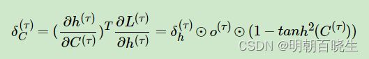
      3.3 最后一个时刻的

              

 这里面要注意这里的

    证明一下第二项，主要应用到微分的两个性质,以及微分和迹的关系：

   

     ... 公式1： 微分和迹的关系

       

     因为

    

   

           

     带入上面公式1：

      

           

    所以

3.4   链式求导过程

       求导结果：

 

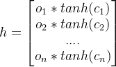
  这里详解一下推导过程：

  这是一个符合函数求导：先把h 写成向量形成

 ------------------------------------------------------------   

 第一项： 

             

         

         

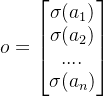
        设 

           则    

 

            其中：（利用矩阵求导的定义法 分子布局原理）

                     是一个对角矩阵

                  

                 

                 

                 几个连乘起来就是第一项

               

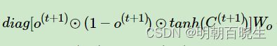
第二项

    

   

   

  

参考：

   

其中：

 

 

其它也是相似，就有了上面的求导结果

---

四  为什么能解决梯度消失

    

     4.1 RNN 梯度消失的原理

                ,复旦大学邱锡鹏书里面 有更加详细的解释，通过极大假设：

在梯度计算中存在梯度的k 次方连乘 ，导致 梯度消失原理。

    4.2  LSTM 解决梯度消失 解释1：

            通过上面公式发现梯度计算中是加法运算，不存在连乘计算，

            极大概率降低了梯度消失的现象。

    4.3  LSTM 解决梯度 消失解释2：

              记忆单元c  作用相当于ResNet的残差部分.  

   比如 时候,,不会存在梯度消失。

       

---

五 模型的搭建

   

    我们最后发现：

     的维度必须一致，都是hidden_size

    通过,则  最后一个维度也必须是hidden_size

    

# -*- coding: utf-8 -*-
"""
Created on Thu Aug  3 15:11:19 2023

@author: chengxf2
"""

# -*- coding: utf-8 -*-
"""
Created on Wed Aug  2 15:34:25 2023

@author: chengxf2
"""

import torch
from torch import nn
from d21 import torch as d21


def normal(shape,devices):
    
    data = torch.randn(size= shape, device=devices)*0.01
    
    return data


def get_lstm_params(input_size, hidden_size,categorize_size,devices):
    


    
    #隐藏门参数
    W_xf= normal((input_size, hidden_size), devices)
    W_hf = normal((hidden_size, hidden_size),devices)
    b_f = torch.zeros(hidden_size,devices)
    
    #输入门参数
    W_xi= normal((input_size, hidden_size), devices)
    W_hi = normal((hidden_size, hidden_size),devices)
    b_i = torch.zeros(hidden_size,devices)
    

    
    #输出门参数
    W_xo= normal((input_size, hidden_size), devices)
    W_ho = normal((hidden_size, hidden_size),devices)
    b_o = torch.zeros(hidden_size,devices)
    
    #临时记忆单元
    W_xc= normal((input_size, hidden_size), devices)
    W_hc = normal((hidden_size, hidden_size),devices)
    b_c = torch.zeros(hidden_size,devices)
    
    #最终分类结果参数
    W_hq = normal((hidden_size, categorize_size), devices)
    b_q = torch.zeros(categorize_size,devices)
    
    
    params =[
        W_xf,W_hf,b_f,
        W_xi,W_hi,b_i,
        W_xo,W_ho,b_o,
        W_xc,W_hc,b_c,
        W_hq,b_q]
    
    for param in params:
        
        param.requires_grad_(True)
        
    return params

def init_lstm_state(batch_size, hidden_size, devices):
    
    cell_init = torch.zeros((batch_size, hidden_size),device=devices)
    hidden_init = torch.zeros((batch_size, hidden_size),device=devices)
    
    return (cell_init, hidden_init)


def lstm(inputs, state, params):
    [
        W_xf,W_hf,b_f,
        W_xi,W_hi,b_i,
        W_xo,W_ho,b_o,
        W_xc,W_hc,b_c,
        W_hq,b_q] = params    
    
    (H,C) = state
    outputs= []
    
    for x in inputs:
        
        #input gate
        I = torch.sigmoid((x@W_xi)+(H@W_hi)+b_i)
        F = torch.sigmoid((x@W_xf)+(H@W_hf)+b_f)
        O = torch.sigmoid((x@W_xo)+(H@W_ho)+b_o)
        
        C_tmp = torch.tanh((x@W_xc)+(H@W_hc)+b_c)
        C = F*C+I*C_tmp
        
        H = O*torch.tanh(C)
        Y = (H@W_hq)+b_q
        
        outputs.append(Y)
        
    return torch.cat(outputs, dim=0),(H,C)
        
    

def main():
    batch_size,num_steps =32, 35
    train_iter, cocab= d21.load_data_time_machine(batch_size, num_steps)

    

if __name__ == "__main__":
    
     main()

---

 参考

 

CSDN

https://www.cnblogs.com/pinard/p/6519110.html

57 长短期记忆网络（LSTM）【动手学深度学习v2】_哔哩哔哩_bilibili