DipC 构建基因组 3D 结构(学习笔记)
背景
本文主要记录了 DipC 数据的复现过程、学习笔记及注意事项。
目录
- 下载 SRA 数据
- 使用 SRA Toolkit 转换 SRA 数据为 Fastq 格式
- 使用 bwa 比对测序数据
- 使用 Hickit 计算样本的基因组 3D 结构
- 使用散点图展示 3D 结构
- 计算 3D 结构重复模拟的稳定性
- 其他
步骤
1. 下载 SRA 数据
1.1 从 NCBI 网站下载 SRA 数据(桌面操作)
根据 https://github.com/tanlongzhi/dip-c 的 README.md,下载 PRJNA607329 项目(Mouse Brain, https://www.ncbi.nlm.nih.gov/sra/PRJNA607329)中 “Hippocampus P56 CASTxB6 Cell 132” 的测序数据作为后续分析的起始数据。该测序数据的 SRR 编号为 SRR11120618,下载格式为 “SRA Lite”。下载路径为 https://sra-downloadb.be-md.ncbi.nlm.nih.gov/sos5/sra-pub-zq-16/SRR011/11120/SRR11120618/SRR11120618.lite.1。然后使用 SRA-Toolkit 将数据转化为 Fastq 格式。
SRA 数据分为标准格式(Normalized)和简化格式(Lite)两种。其中,Lite 简化了 Normalized 格式中 reads 的质量分数(quality score),仅区分 “合格” 与 “不合格”,所以数据大小较小,节省数据的传输时间。
1.2 使用 SRA Toolkit 下载SRA数据(命令行操作)
SRA Toolkit是NCBI SRA数据库文件下载和转换为Fastq的工具。从Github下载适配系统的SRA-Toolkit(https://github.com/ncbi/sra-tools/wiki/02.-Installing-SRA-Toolkit)。或者通过下面命令获取(在当前目录下生成名为sratoolkit.tar.gz的文件)并解压(在当前目录下生成名为sratoolkit.3.0.7-ubuntu64的文件夹)。
$ wget --output-document sratoolkit.tar.gz https://ftp-trace.ncbi.nlm.nih.gov/sra/sdk/current/ sratoolkit.current-ubuntu64.tar.gz

$ tar -vxzf sratoolkit.tar.gz
使用 SRA Toolkit 的 prefetch 模块下载 SRA 数据,由于 SRA 数据较大,prefetch 模块建议与 nohup 和 & 连用,避免意外中断。SRA Toolkit 将在指定目录(-O DipC_SRR11120618/)内下载 SRR11120618 数据(默认下载标准格式数据)。下载完成后生成 SRR11120618.sra 文件。
$ nohup sratoolkit.3.0.7-ubuntu64/bin/prefetch –O DipC_SRR11120618/SRR11120618 &
2. 使用 SRA Toolkit 转换 SRA 数据为 Fastq 格式
使用 SRA Toolkit 的 fasterq-dump 模块将 SRR11120618.lite.1 数据转换为 Fastq 格式,在指定目录(-O DipC_SRR11120618)下生成 SRR11120618.lite.1_1.fastq 和 SRR11120618.lite.1_2. fastq 文件。
$ sratoolkit.3.0.7-ubuntu64/bin/fastq-dump --split-3 –O DipC_SRR11120618 DipC_SRR11120618/SRR11120618.lite.1
    --split-3    将双端测序分为两份,放在不同的文件,但是对于一方有而一方没有的 reads 会单独放在一个文件夹里。
3. 使用 bwa 比对测序数据
首先,使用bwa构建参考基因组(mm10.fa)的 FM-index。构建完成后,在当前目录下会生成 .amb、.ann、.bwt、.pac、.sa 后缀的 index 文件。
$ bwa index mm10_reference/GenomeFastq_and_BWAIndex/mm10.fa
然后,使用 bwa 的 mem 算法对 reads 进行比对。bwa 包含 bwa-backtrack、bwa-sw、bwa-mem 三种算法,一般情况推荐使用 mem 算法。
$ bwa mem -t 40 mm10_reference/GenomeFastq_and_BWAIndex/mm10.fa DipC_SRR11120618/SRR11120618.lite.1_1.fastq DipC_SRR11120618/SRR11120618.lite.1_2.fastq | gzip > SRR11120618.aln.sam.gz
    -t 40   表示 bwa 比对时使用 40 个线程。
4. 使用 Hickit 计算样本的基因组 3D 结构
4.1 下载并安装 Hickit
从 GitHub 上下载 Hickit(https://github.com/lh3/hickit/releases/download/v0.1.1/hickit-0.1.1_x64-linux.tar.bz2),得到压缩包 hickit-0.1.1_x64-linux.tar。注意,要从 Releases 板块下载,不能从 GitHub 的 Code 下载(Code-> Download ZIP),否则会缺失 hickit 和 k8 文件。下载完毕后使用 tar 解压 Hickit,在当前目录下生成 hickit-0.1.1_x64-linux 文件夹。
$ tar -jxf hickit-0.1.1_x64-linux.tar.bz2
	-x  解压
	-j  解压具有 bz2 属性的文件
	-f  使文件名字命名输出文件
4.2 根据比对结果计算连接
以比对结果(.aln.sam.gz)作为输入,使用 Hickit 的 hickit.js 文件计算基因组不同片段之间的连接情况,输出 seg 格式文件。虽然 SRR11120618 样本是二倍体小鼠,但由于本人后续研究项目材料为纯合小鼠,所以这里将 SRR11120618 样本视为单倍体小鼠处理,跳过了 Hickit 对连接定相(-v)与填补(-u)的步骤,并且删除样本中与 Y 染色体相关的连接(chronly -y)。
$ hickit-0.1.1_x64-linux/k8 hickit-0.1.1_x64-linux/hickit.js sam2seg DipC_SRR11120618/SRR11120618.aln.sam.gz > DipC_SRR11120618/SRR11120618.contacts.seg
	sam2seg 	根据比对结果计算连接

$ hickit-0.1.1_x64-linux/k8 hickit-0.1.1_x64-linux/hickit.js chronly -y DipC_SRR11120618/SRR11120618.contacts.seg | gzip > DipC_SRR11120618/SRR11120618.contacts.seg.gz
	chronly 	仅保留染色体上的连接(filters out non-chromosomal contigs)
	-y      	删除样本中与 Y 染色体相关的连接
将连接结果由 seg 格式转化为 pairs 格式(必须),并使用 bgzip 压缩(可选)。
$ hickit-0.1.1_x64-linux/hickit -i DipC_SRR11120618/SRR11120618.contacts.seg.gz -o - | bgzip > DipC_SRR11120618/SRR11120618.contacts.pairs.gz
    -i      输入文件的路径,支持 seg 或 pairs 格式的文件作为输入
    -o      输出文件的路径
    bgzip   将文件压缩为 BGZF 格式文件
注意,由于 DipC 在转换 Hickit 输出数据为 DipC 的输入格式文件时,只支持 bgzip 的压缩格式(BGZF),不支持 gzip 的压缩格式。所以后续如果使用 DipC 软件,则 必须 要使用 bgzip 压缩。另外,bgzip 是 htslib 软件(samtools系列)下的一个模块,需要先下载 htslib 软件(conda install -c bioconda htslib)。下载完成后,即可在命令行直接键入 bgzip 进行调用。
4.3 通过连接计算基因组 3D 结构
$ hickit-0.1.1_x64-linux/hickit -i DipC_SRR11120618/SRR11120618.contacts.pairs.gz -r1m -c1 -r10m -c5 -b4m -b1m -O DipC_SRR11120618/SRR11120618.haplo.1m.3dg -b200k -O DipC_SRR11120618/SRR11120618.haplo.200k.3dg -D5 -b50k -O DipC_SRR11120618/SRR11120618.haplo.50k.3dg
    -c          filter pairs if within -r, #neighbors
    -r          radius [default=10m]
    -b          3D modeling at NUM resolution
    -D          filter contacts with large 3D distance
    -S          separate homologous chromosomes
    -O          write the 3D model to FILE
-r1m 表示半径为 1m
-c5 表示删除指定范围内(-r)连接数小于 5 的片段(bin)
-r 和 -c 是配套的参数,用于过滤孤立连接(isolated contact)的区间。Hickit 将区间内 Contact Num 不符合条件的区间视为孤立区间,这些区间由于连接数较少,提供的信息不一定准确,不用于后续 3D 结构搭建。上述命令中 Hickit 进行了两轮筛选 “–r1m –c1” 与 “–r10m –c5”。第一轮 “–r1m –c1” 表示过滤 1Mb 范围内 Contact Num 小于 1 的 Bin,即过滤以 1MB 为分辨率中不含 Contact 的 Bin。第二轮为 “–r10m –c5”,过滤 10Mb 范围内 Contact Num 小于 5 的 Bin。第二次过滤是为了避免估算局部缺失过多的结构,如 10MB 范围内仅有 1 个连接。
-S 表示数据为二倍体,hickit 计算 3D 结构时将区分父母本的染色体。如果是单倍体,则不能使用 -S 参数,否则会报错 “hickit: main.c:188: main: Assertion `(m->cols & 0x3c) == 0x3c’ failed.”。(“if it is haploid data, don’t use -S; if it is diploid data, run hickit.js sam2seg -v and impute with hickit -u” by lh, Hickit GitHub: Working on my haploid dataset · Issue #3)
-b4m 表示搭建的 3D 模型的分辨率为 10MB。上述命令对模型进行了 4 轮不同分辨率的迭代(-b4m, -b1m, -b200m, -b50k)。在进行多轮迭代时,模型要求分辨率逐步提高(applies five rounds of 3D modeling (the four -b actions) with each at a higher resolution),并且 Hickit 会以低分辨率的结构为基础计算高分辨率的结构。注意,当分辨率降到 100k 以下时,Hickit 教程中建议使用者添加 -D 参数。-D 的功能是去掉远距离的 Contact,个人认为是避免细节被远距离 Contact 干扰。
Multiple particle sizes can be specified so that the genome structure calculation uses a hierarchical protocol, calculating a low resolution structure first and then basing the next, finer resolution stage on the output of the previous stage. Hierarchical particle sizes need not be used, but they make the calculation more robust.(by nuc_dynamics, README.txt)
5. 使用散点图展示 3D 结构
3dg 格式文件中记录了 Hickit 计算的染色体片段在 3D 空间的坐标,可以直接通过 Python 脚本绘制散点图(下图)。其中不同颜色表示不同的染色体。
import pandas as pd
import matplotlib.pyplot as plt

data_path = "DipC_SRR11120618/new/SRR11120618.haplo.1m.3dg"
data_3d = pd.DataFrame()
with open(data_path, 'r') as d:
    for row in d.readlines():
        if not row.startswith('#'):
            row = row.strip().split('\t')
            row = pd.DataFrame({
                'chrID': [row[0].strip('chr')],
                'BinID': [int(row[1])],
                'x': [float(row[2])],
                'y': [float(row[3])],
                'z': [float(row[4])]})
            data_3d = pd.concat([data_3d, row], axis=0)
data_3d['chrID'] = data_3d['chrID'].replace('X', 20)
data_3d['chrID'] = data_3d['chrID'].apply(lambda x: int(x))

# Creating figure
fig = plt.figure(figsize=(10, 7))
ax = plt.axes(projection="3d")
my_cmap = plt.get_cmap('hsv')
sctt = ax.scatter3D(data_3d['x'], data_3d['y'], data_3d['z'], c=data_3d['chrID'], cmap=my_cmap)
plt.title("SRR11120618  Resolution=1MB ")
plt.show()

注意!由于 SRR11120618 数据是 二倍体非纯合 小鼠的单细胞测序结果,但本实验没有按照作者教程内容对测序数据通过 SNP 进行定向,区分连接所在染色体的父母本来源,而是将数据按照单倍型的模式输入并建模。所以上图结果并非真实的细胞内染色体 3D 构象,仅是 Hickit 根据连接情况模拟出的可能构象。
6. 计算 3D 结构重复模拟的稳定性
6.1 Hickit 重复建模
首先,使用 Hickit 进行三次 3D 建模。由于随机种子不同(-s random number seed),所以模型的起始状态不同。
import subprocess
for r in range(3):
    subprocess.Popen(' hickit-0.1.1_x64-linux/hickit -s{0} -i DipC_SRR11120618/SRR11120618.contacts.pairs.gz -r1m -c1 -r10m -c5 -b1m -O DipC_SRR11120618/SRR11120618.haplo.seed{0}.1m.3dg'.format(r), shell=True)
6.2 下载 DipC 并转换数据格式
Hickit 不包含计算不同模拟之间稳定性的功能,需要调用 DipC 的 align 模块来实现。下面将下载 DipC,然后将数据转换为 DipC 支持的输入格式。注意!DipC 的运行环境为 Python2.7。使用 Python3 运行会报错(参见 DipC Github: issue #55, ‘str’ error when convert 3dg file to cif file),具体错误如下。
Traceback (most recent call last):
  File "../dip-c/dip-c", line 130, in <module>
    main()
  File ".../dip-c/dip-c", line 75, in main
    return_value = color.color(sys.argv[1:])
  File ".../dip-c/color.py", line 218, in color
    g3d_data = file_to_g3d_data(open(args[0], "rb"))
  File ".../dip-c/classes.py", line 1427, in file_to_g3d_data
    g3d_data.add_g3d_particle(string_to_g3d_particle(g3d_file_line.strip()))
  File ".../dip-c/classes.py", line 1214, in string_to_g3d_particle
    hom_name, ref_locus, x, y, z = g3d_particle_string.split("\t")
TypeError: a bytes-like object is required, not 'str'
由于 DipC 是通过 Python 脚本编写,所以从 GitHub 的 Code 下载(Code-> Download ZIP)并解压后即可使用。Hickit 的输出格式与 DipC 的输入格式并不兼容,需要使用 DipC 内置脚本(hickit_3dg_to_3dg_rescale_unit.sh)进行格式转换。
import subprocess
for r in range(3):
    subprocess.Popen(
        'dip-c-master/scripts/hickit_3dg_to_3dg_rescale_unit.sh DipC_SRR11120618/SRR11120618.haplo.seed{0}.1m.3dg'.format(r), shell=True)
6.3 使用 align 模块分析稳定性
DipC 通过计算 RMSD(Root Mean Square Deviation)值来评估不同模型之间的相似度,进而判定不同模拟之间的稳定性。RMSD 反映的是数据偏离平均值的程度,常用于蛋白质结构解析及分子动力学模拟中,衡量原子偏离比对位置的程度。注意!DipC 调用 Python 的 rmsd 包来计算 RMSD 值,所以需要先安装依赖(rmsd)。
$ pip install rmsd
$ dip-c-master/dip-c align DipC_SRR11120618/SRR11120618.haplo.seed[0-2].1m.3dg > DipC_SRR11120618/SRR11120618.haplo.1m.rmsd
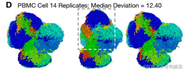
DipC 将计算所有模型之间的偏差,输出文件内包含了每个片段的 RMSD 值,标准输出包含了不同对模型间整体的 RMSD 值。SRR11120618 样本 3D 模型的 RMSD 的中位数为 1.242,均方差为 2.089。DipC 文章中不同重复之间的 RMSD 偏差在 1 左右(与本实验计算结果相似),但有 3 个样本的偏差超过了 10。这些细胞的 3D 结构重复之间偏差超过 10 的原因是其结构非圆形,而是多叶(lobes)结构,不同叶之间建模算法允许其扭转,进而导致不同重复间差异较大(下图)。
7. 其他
7.1 DipC 与 Hickit 的构建 3D 结构算法的异同
DipC 和 Hickit 构建染色体 3D 结构都是基于 nuc_dynamics 算法,但在处理无连接的染色体片段时存在差异。DipC 和 nuc_dynamics 使用所有片段进行建模,其中无连接信息的片段被视为 large, free-floating loops。然后再删除低连接区、无连接区的 3D 结构(通过 clean 模块),而 Hickit 则是将无连接的片段合并或删除。即 DipC、nuc_dynamics 是先建模后删除,Hickit 是先删除后建模。从具体样本的 3D 结构模拟结果来看,DipC 构建的 3D 模型较连续,但存在异常结构(下图 1);Hickit 构建的模型片段化,但结构较为合理(下图 2)。DipC 将蓝色染色体分为 3 个部分,不同区块之间由刚性结构连接,而非柔性连接,所以此结构并非因片段缺少连接而产生,大概率为 DipC 错误模拟而导致。因此,DipC 作者谭隆志更推荐使用 Hickit 算法构建染色体的 3D 结构。
DipC 模拟的 2 号染色体 3D 结构

Hickit 模拟的 2 号染色体 3D 结构

原文参见 Dip-c Github Issue #17: Dip-c vs hickit for preprocessing
It seems to me that in both cases, you’re observing aberrantly stretched backbones rather than free-floating loops. (Free-floating loops are soft and bendy; these are very straight.) This seems to be the result of incorrect imputation, mistakenly assigning intrahomologous contacts to interhomologous contacts.
In dip-c/nuc_dynamics, regions that harbor no contacts (and therefore no constraints) will float away from the nucleus, forming large, free-floating loops either outside or on the surface of the nucleus. Although these regions are later deleted (for example, by dip-c clean3), such floating behavior is certainly incorrect.
The seemingly “noncontiguous” hickit models are in fact a clever design of adaptive genomic resolution, where 3D particles (20 kb each, in this case) that harbor no contacts are automatically merged with nearby particles to form larger particles (40 kb each, or larger). This can be a better way to handle repetitive regions such as the centromeres, and has nothing to do with 3D vs 2D imputation. This mode can be turned off to produce more dip-c-/nuc_dynamics-like models by the hickit -M option.
原文参见 Hickit Github Issue #5: Analyzing diploid mESC data from Nagano et al. (2017)
Regarding the loss of many 3D particles in your 20-kb structure, according to my understanding (@lh3 please correct me if I got it wrong), this repo handles particles with no contacts by removing/merging them. This is different from the behavior of dip-c and nuc_dynamics, where contact-poor particles are carried along during 3D modeling, and removed later but only in large regions (e.g. very few contacts in its 1-Mb neighborhood) or manually filtered out later by large RMSD between replicates.
In other words, when the resolution is set too high for the number of contacts in the given single cell, this repo starts to discard 3D particles, while dip-c and nuc_dynamics generate floppy 3D structures with large RMSD. Anyways it’s a sign to use a lower resolution.
7.2 DipC 不适用于 Bulk HiC 的原因
因为 Bulk 数据反应的是多个细胞内的平均连接情况,无法通过单一 3D 结构来描述。所以 DipC 无法构建基于 Bulk HiC 连接数据的 3D 结构。但除了 3D 模块和单倍型填补模块,其余模块 Hickit 可以正常应用于 Bulk HiC 数据。
原文参见 Hickit Github Issue #3: Working on my haploid dataset
Here the 3D modeling function of hickit, which is similar to that in nuc_dynamics and in Nagano et al. 2017, seeks a 3D genome structure that satisfies nearly all contacts of a contact map. In bulk Hi-C, however, the contact map is an average of many cells with different 3D structures. It is impossible to find a single structure that satisfies nearly all these contacts. You can of course still use other functions of hickit, for example extraction of contacts and their haplotype information from sequencing reads, on bulk Hi-C. It’s only haplotype imputation and 3D modeling that doesn’t apply to bulk.