线性回归＋MK趋势分析对1980-2020全球洪灾受灾情况进行分析

1、数据

        40年的洪灾统计数据，包含八个相关因子：

2、线性回归

     直接在excel里生成线性趋势线，用拟合函数作为线性函数：

3、MK趋势分析＋泰森斜率MATLAB源码：

MATLAB泰森斜率+MK趋势分析函数代码-其它文档类资源-CSDN下载

function [taub tau h sig Z S sigma sen n senplot CIlower CIupper D Dall C3 nsigma] = ktaub(datain, alpha, wantplot)
    
    try
        %% Check MATLAB version for compatibility
        % Added this version trap since the most common comment I get is
        % they syntax is in error.  So far when people get this error it's
        % because they are using an old version of matlab that does not
        % accept some of the variable names in this function.
        % 7/23/2011 - JJB
        vmat = regexp(version,'\d+','match');
        vr = [str2double(vmat{1}) str2double(vmat{2})];
        
        if vr(1) == 7
            if vr(2) >=9 || vr(1) > 7
                % Then matlab version should work
            else
                txt = 'Your version of matlab is %s. \nYou need at least version 7.9 to run.\n Some of the syntax will not parse correctly.';
                warning(txt,version)
            end
        end
    catch msg
        error('Matlab version is way too old to run this function.');
    end
    
    
    % wantplot is a flag to create a figure or not default set to no
    if exist('wantplot','var') == 0
        % user didn't provide assume zero (i.e. no plot)
        wantplot = 0;
    end
    % Data are assumed to be in long columns, hence 'sortrows'
    sorted = sortrows(datain,1);
    % remove any NaNs, if data are missing they should not be included as
    % NaNs.
    sorted(any(isnan(sorted),2),:) = [];
    
    % return n after removing any NaNs
    n = size(sorted,1);
    
    % set to NaN if trend is not significant
    senplot = NaN;
    
    % extract out the data
    row1 = sorted(:,1)';
    row2 = sorted(:,2)';
    
    clear sorted;
    
    L1 = length(row1);
    L2 = L1 - 1;
    
    % find ties
    ro1 = sort(row1)';
    ro2 = sort(row2)';
    [~,b] = unique(ro1);
    [~,e] = unique(ro2);
    
    clear a c d f ro1 ro2;
    
    % correcting loss of first value using diff on with unique
    if b(1,1) > 1
        ta = b(1,1);
    else
        ta = 1;
    end
    if e(1,1) > 1
        tb = e(1,1);
    else
        tb = 1;
    end
    bdiff = [ta; diff(b)];
    ediff = [tb; diff(e)];
    
    clear ta tb b e;
    
    %% Determine ties used for computing adjusted variance
    tp = sum(bdiff .* (bdiff - 1) .* (2 .* bdiff + 5));
    uq = sum(ediff .* (ediff - 1) .* (2 .* ediff + 5));
    
    % modified 12/1/2008
    % adjustments when time index has multiple observations
    d1 = 9 * L1 * (L1-1) * (L1-2);
    tu1 = sum(bdiff .* (bdiff - 1) .* (bdiff - 2)) * sum(ediff .* (ediff - 1) .* (ediff - 2)) / d1;
    d2 = 2 * L1 * (L1-1);
    tu2 = sum(bdiff .* (bdiff - 1)) * sum(ediff .* (ediff -1)) / d2;
    
    % ties used for adjusting denominator in Tau
    t1a = (sum(bdiff .* (bdiff - 1))) / 2;
    t2a = (sum(ediff .* (ediff - 1))) / 2;
    
    % create matricies to be used for substituting values as indicies
    m1 = repmat((1:L2)',[1 L2]);
    m2 = repmat((2:L1)',[1 L2])';
    
    % populate matrixes for analysis
    A1 = triu(row1(m1));
    A2 = triu(row1(m2));
    B1 = triu(row2(m1));
    B2 = triu(row2(m2));
    
    clear m1 m2 row1 row2;
    
    % Perform pair comparison and convert to sign
    A = sign(A1 - A2);
    B = sign(B1 - B2);
    
    %% Perform operations to calculate Sen's Slope 
    % Median of rate of change among all data points- CLD added 5/3/2006
    A3 = reshape((A1 - A2),L2*L2,1);
    B3 = reshape((B1 - B2),L2*L2,1);
    a = find(A3~=0);
    C3 = sort(B3(a)./A3(a));
    sen = median(C3);
    
    clear A1 A2 B1 B2 A3 B3 a;
    
    %% Evaluate concordant and discordant
    % +1 = concordant
    % -1 = discordant
    %  0 = tie
    C = A.*B;
    % Compute S
    S = sum(sum(C,2));
    
    clear A B C;
    
    % Calculate denominator with ties removed Tau-b
    D = sqrt(((.5*L1*(L1-1))-t1a)*((.5*L1*(L1-1))-t2a));
    % Calcuation denominator no ties removed Tau
    Dall = L1 * (L1 - 1) / 2;
    
    % (modified 12/1/2008: added tau)
    tau = S / Dall;
    
    taub = S / D;
    
    % adjust for normal approximations and continuity
    if S > 0
        s = S -1;
    elseif S < 0
        s = S + 1;
    elseif S == 0
        s = 0;
    elseif isnan(S)
        error('ErrorTrend:ktaub', 'This function cannot process NaNs. \nPlease remove data records with NaNs.\n');
    end
    
    %% Test for abnormalities in data
    % Certain conditions can occur that potentially invalidate this
    % statistic. Conditional statements conduct some tests and provide the
    % user some feedback.
    if S==1
        % Notify user continuity correction is setting S = 0
        fprintf('\nTaub Message:  When absolute value S=1,');
        fprintf('\n               Continuity correction is setting S = 0.');
        fprintf('\n               This will affect calculated significance.\n');
    end
    
    % compute square-root of variance with all ties accounted for in time
    % index and in observation values. - JJB 12/1/2008
    sigma = sqrt(((L1*(L1-1)*(2*L1 + 5) - tp - uq) / 18) + tu1 + tu2);
    
    % nsigma is used if slope is zero and determined significant.  It is
    % hypothesized that all ties can be represented as an equal number of
    % postive and negative slopes.
    nsigma = sqrt(L1*(L1-1)*(2*L1+5));
    
    Z = s / sigma;
    
    % Estimate confidence intervals of Sen's slope
    %      The next line requires STATISTICS Toolbox (norminv)
    %      Zup is a 2-tail Z (i.e. alpha/2)
    %
    % Hollander, M. and Wolfe, D. 1973, Nonparametric statistical methods, 
    % Wiley, New York. Chapter 9 (Regression problems involving slope), 
    %      Section 3 (A distribution-free confidence interval based on the 
    %      Theil test; p. 207 - 208)
    
    Zup = norminv(1-alpha/2,0,1);
    Calpha = Zup * sigma;
    Nprime = length(C3);
    M1 = (Nprime - Calpha)/2;
    M2 = (Nprime + Calpha)/2 + 1;
    % 2-tail limits
    CIlower = interp1q((1:Nprime),C3,M1);
    CIupper = interp1q((1:Nprime),C3,M2);
    
    %     clear M1 M2 NPrime Zup Calpha
    
    % h = 1 : means significance
    % h = 0 : means not significant (i.e. sig < z(sig))
    if s==0
        % Not possible to be 100% certain, force S = 1 and compute p-value
        % using sigma.
        [h, sig] = ztest(1,0,sigma,alpha);
        fprintf('\nTaub Message: S = 0. P-value cannot = 100-percent. ');
        fprintf('\n              P-value is adjusted using S = 1 and should be reported as p > %1.5f.\n',sig);
        if sen~=0
            fprintf('\nTaub Message: A non-zero Sens slope occurred when S =0.');
            fprintf('\n              This is not an error, more a notification.');
            fprintf('\n              This anomaly may occur because the median may be computed');
            fprintf('\n              on one value equal to zero and one non-zero, etc.\n');
        end
    else
        [h, sig] = ztest(s,0,sigma,alpha);
    end
    
    % Notify for Sens slope = 0 but is determined significant
    if h==1 && sen==0
        [hh, nsig] = ztest(s,0,nsigma,alpha);
        fprintf('\nTaub Message:  There was a significant trend = 0 found.\n');
        fprintf('               Retested with ties set to equal number of positve and negative values.\n');
        fprintf('               New p-value = %1.5f',nsig);
        if hh==1
            fprintf('.  However trend still found to be significant.\n');
        else
            fprintf(', but trend is not found to be significant.\n');
        end
    end
    
    %% Plotting routine
    % Below is a very simplistic plotting routine to plot the Sen slope if
    % the significance is less than 0.05. Uncomment or delete at your
    % leisure.
    if sig<=alpha && wantplot ~= 0  %A plotting example CLD added 5/3/2006
        % Revised plotting 6/14/2011 - JJB
        % Plots the slopes using the median value as the focus point for
        % all three slopes (Sen's and confidence slopes). Is this the
        % correct method? Don't know but seems reasonable. - JJB 6/15/2011
        hold on
        %generate points to represent median slope
        %zero time for the calculation is the first time point
        vv = median(datain(:,2));
        
        middata = datain(round(length(datain)/2),1);
        slope = vv + sen*(datain(:,1)-middata);
        senplot = [datain(:,1) slope];
        
        plot(datain(:,1),datain(:,2),'o')
        plot(datain(:,1),slope,'-')
        
        % add confidence intervals
        slope = vv + CIlower*(datain(:,1)-middata);
        plot(datain(:,1),slope,'--');
        
        slope = vv + CIupper*(datain(:,1)-middata);
        plot(datain(:,1),slope,'--');
        box on
        grid on
        hold off
        %         pause
    end
end

调用：

clc;clear
year = (1970:2020)';
data = xlsread('D:\FLOOD\new_data\统计法\M-K趋势分析.xlsx','year','F2:F52');
ts = [year data];
[taub, tau, h, sig, Z, S, sigma, sen] = ktaub(ts,0.05,0);
slope = sen;
p = sig;
zscore = Z;

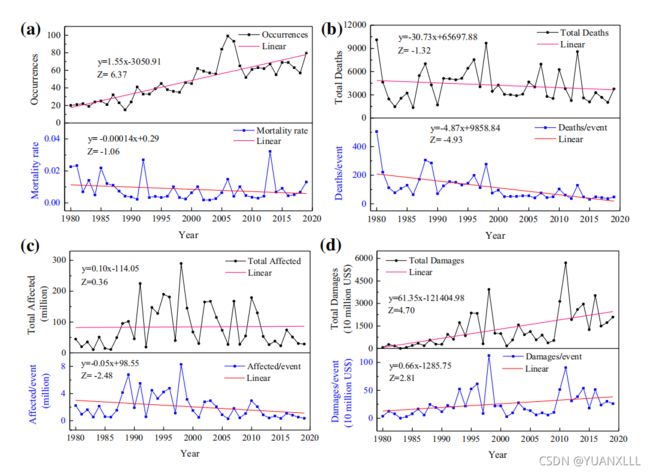
4、分析结果：

（发生次数、死亡率）、（总死亡人数、平均每次事件的死亡人数）、（总影响人数、平均每次事件的影响人数）、（总经济损失、平均每次事件的损失）

成果类似下图：来自论文 https://doi.org/10.1007/s11069-021-04798-3