AdaBins：Depth Estimation using Adaptive Bins

文章目录

• 一、AdaBins处理的问题
• 二、AdaBins整体架构
  • 1.MVIT
  • 2.个人理解

---

一、AdaBins处理的问题？

并提出了全局信息处理如何帮助改进整体深度估计的问题。
提出了一种基于变换的体系结构块，该结构块将深度范围划分为每个图像自适应地估计其中心值的子块。最终深度值估计为面元中心的线性组合。

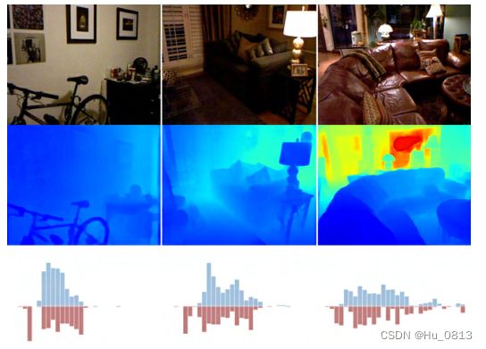
 这是论文中给的GT深度分布图和预测的深度分布图，如果两者在深度分布上能够尽可能达到一致的话，其实就已经将损失降到了一定的程度

二、AdaBins整体架构

文章采用传统的编解码模块 Encoder：EfficientNet B5 （这里不做介绍），Decoder得到的feature-map 进入本文中提到的mVIT模块  这也是本文中的核心所在

1.MVIT

对于decoder得到的feature-map channel=128 通过2个分支，我们先看一下底部的Transformer部分

class PatchTransformerEncoder(nn.Module):
    def __init__(self, in_channels, patch_size=10, embedding_dim=128, num_heads=4):
        super(PatchTransformerEncoder, self).__init__()
        encoder_layers = nn.TransformerEncoderLayer(embedding_dim, num_heads, dim_feedforward=1024)
        self.transformer_encoder = nn.TransformerEncoder(encoder_layers, num_layers=4)  # takes shape S,N,E

        self.embedding_convPxP = nn.Conv2d(in_channels, embedding_dim,
                                           kernel_size=patch_size, stride=patch_size, padding=0)

        self.positional_encodings = nn.Parameter(torch.rand(500, embedding_dim), requires_grad=True)

    def forward(self, x):
        embeddings = self.embedding_convPxP(x).flatten(2)  # .shape = n,c,s = n, embedding_dim, s
        # embeddings = nn.functional.pad(embeddings, (1,0))  # extra special token at start ?
        embeddings = embeddings + self.positional_encodings[:embeddings.shape[2], :].T.unsqueeze(0)

        # change to S,N,E format required by transformer
        embeddings = embeddings.permute(2, 0, 1)
        x = self.transformer_encoder(embeddings)  # .shape = S, N, E
        return x

 作者使用了一个简化版的vit ，feature_map x通过一个卷积嵌入，得到 Transformer输入需要的token  

与vit类似的操作，加了一个位置编码，并将其转化输入进入4层transformer Encoder层，详细步骤可以看一下vit代码，得到的 x：SxBx128     demo: S=15*20=300

Bin widths = x[0,:]  # 1x128

query = x[1:128+1,:,:] # 128xBx128 

query经过permute -->Bx128x128  #后面的128是维度

如果将此时的query再次经过permute(0,2,1) 此时中间的128是维度

接着看mvit上部分支 feature map经过3*3特征图经过结果与query进行矩阵相乘，非点乘

feature-map.T 与 query进行矩阵相乘 得到 range_attention_maps .size=B x (hxw) x 128

看一下此时的range_attention_map图左与最终图右区别 

  

接着将上述的map图通过3个linear层，得到 bin_widths_normed = 1*256

range_attention_map经过卷积层得到与bin_widths_normed相同的维度1x256x240x320

out=range_attention_map  

bin_widths可以通过最大最小值计算出  并*bin_widths_normed将 bin 划分为256份

通过取bin的中间center进行回归操作，以最小深度在左侧添加一个深度bin, 此时bin有257份

通过torch.cumsum 可以得到深度bin的边界（从min_depth开始）

详情参考代码

bin_widths = (self.max_val - self.min_val) * bin_widths_normed  
bin_widths = nn.functional.pad(bin_widths, (1, 0), mode='constant', value=self.min_val)
bin_edges = torch.cumsum(bin_widths, dim=1)  #torch.cumsum 第一列不变，其他每一列累加至最后一列
centers = 0.5 * (bin_edges[:, :-1] + bin_edges[:, 1:])
# bin_edges[:,:-1]指的是从第一个元素到倒数第二个元素， bin_edges[:,1:]指的是从第二个元素到最后一个元素
n, dout = centers.size()
centers = centers.view(n, dout, 1, 1)
pred = torch.sum(out * centers, dim=1, keepdim=True)

2.个人理解

一个图片分成若干个patch之后  将此时的patch进行线性操作，然后经过若干层的自注意力机制之后，此时这个patch是与整张图片通过相似度建立了联系。

比如说 patch1[:,1]是与白色相关的，那整张图片对应位置白色居多的话，那么patch1[:,1]与之点乘 权值就大，其他相应的响应也类似，比如说同样在depth0-depth1深度的响应就会大。

作者通过损失函数的约束，将TRansformer输出结果，聚集于关注深度值

在vit模型中MLP输出的是分类的结果，在本篇论文模型中，输出的是深度的信息 bin

query得到的是全局信息中的不同深度值 如下图所示

 

feature map 与query构成一个 query 与 key 的匹配，之后得到的map[i] 就是深度为query[i]的响应

然后再将深度信息 bin 映射到数据处理中的min_depth-—max_depth 防止伪影，网格的生成，再将再将map中的不同bin的center进行一个平滑处理，就是线性回归

这里损失函数就不再赘述

转载请标注出处

---