从零开始实现神经网络(一)_NN神经网络
参考文章:神经网络介绍
一、神经元
这一神经网络的基本单元,神经元接受输入,对它们进行一些数学运算,并产生一个输出。

这里有三步。
首先,将每个输入(X1)乘以一个权重![]() :
:
![]()
![]()
接下来,将所有加权输入与偏置![]() 相加:
相加:
![]()
最后,总和通过激活函数![]() 传递:
传递:
![]()
激活函数
激活函数用于将无界输入转换为具有良好、可预测形式的输出。常用的激活函数是sigmoid功能:
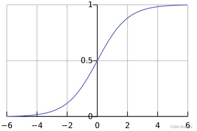
你可以把它想象成,压缩零到负无穷的数字到[-1,0],压缩0到正无穷的数字到[0,1]
举个例子:
这里写成向量形式,假设权重W = {w1,w2} = {0,1},输入X = {x1,x2} = {2,3},偏置b为1。
那么有一下计算:
![]()
![]()
![]()
![]()
下面来实现下代码:
import numpy as np

def sigmoid(x):
  # Our activation function: f(x) = 1 / (1 + e^(-x))
  return 1 / (1 + np.exp(-x))

class Neuron:
  def __init__(self, weights, bias):
    self.weights = weights
    self.bias = bias

  def feedforward(self, inputs):
    # Weight inputs, add bias, then use the activation function
    total = np.dot(self.weights, inputs) + self.bias
    return sigmoid(total)

weights = np.array([0, 1]) # w1 = 0, w2 = 1
bias = 4                   # b = 4
n = Neuron(weights, bias)

x = np.array([2, 3])       # x1 = 2, x2 = 3
print(n.feedforward(x))    # 0.9990889488055994
二. 将神经元组合成神经网络
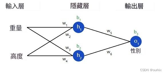
神经网络只不过是一堆连接在一起的神经元。下面是一个简单的神经网络的样子:

该网络有 2 个输入(x1和x2),一个带有 2 个神经元的隐藏层 (ℎ1和ℎ2),以及具有 1 个神经元 (o1).请注意,输入o1是来自ℎ1和h2- 这就是使它成为一个网络的原因。
隐藏层是输入(第一层)和输出(最后一层)之间的任何层。可以有多个隐藏层!
示例:前馈
让我们使用上图的网络,并假设所有神经元具有相同的权重w=[0,1],相同的偏差b=0,以及相同的 S 形激活函数。让h1,h2,o1表示它们所代表的神经元的输出。
如果我们传入输入会发生什么x=[2,3]?
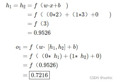
用于输入的神经网络的输出x=[2,3]是0.7216很简单,对吧?
神经网络可以有任意数量的层,这些层中可以有任意数量的神经元。基本思想保持不变:通过网络中的神经元向前馈送输入,以在最后获得输出。为简单起见,在本文的其余部分,我们将继续使用上图的网络。
神经网络的代码实现:
import numpy as np

# ... code from previous section here

class OurNeuralNetwork:
  '''
  A neural network with:
    - 2 inputs
    - a hidden layer with 2 neurons (h1, h2)
    - an output layer with 1 neuron (o1)
  Each neuron has the same weights and bias:
    - w = [0, 1]
    - b = 0
  '''
  def __init__(self):
    weights = np.array([0, 1])
    bias = 0

    # The Neuron class here is from the previous section
    self.h1 = Neuron(weights, bias)
    self.h2 = Neuron(weights, bias)
    self.o1 = Neuron(weights, bias)

  def feedforward(self, x):
    out_h1 = self.h1.feedforward(x)
    out_h2 = self.h2.feedforward(x)

    # The inputs for o1 are the outputs from h1 and h2
    out_o1 = self.o1.feedforward(np.array([out_h1, out_h2]))

    return out_o1

network = OurNeuralNetwork()
x = np.array([2, 3])
print(network.feedforward(x)) # 0.7216325609518421
三. 训练神经网络,第 1 部分
假设我们有以下测量值:
| 名字 | 重量(磅) | 高度(英寸) | 性 |
|---|---|---|---|
| 爱丽丝 | 133 | 65 | F |
| 鲍勃 | 160 | 72 | M |
| 查理 | 152 | 70 | M |
| 黛安娜 | 120 | 60 | F |
让我们训练我们的网络,根据某人的体重和身高预测他们的性别:

我们将用0代表男性,1代表女性,我们还将处理数据以使其更易于使用:
| 名字 | 重量(减去 135) | 高度(减去 66) | 性 |
|---|---|---|---|
| 爱丽丝 | -2 | -1 | 1 |
| 鲍勃 | 25 | 6 | 0 |
| 查理 | 17 | 4 | 0 |
| 黛安娜 | -15 | -6 | 1 |
我随意选择了减去的数值(135和66) 以使数值看起来更好。通常,会按平均值移动。
损失
在我们训练网络之前,我们首先需要一种方法来量化它做得有多“好”,以便它可以尝试做得“更好”。这就是损失所在。
我们将使用均方误差 (MSE) 损失:
![]()
让我们分解一下:
- n是样本数,即4(爱丽丝,鲍勃,查理,戴安娜)。
- y表示要预测的变量,即性别。
- yTrue是变量的真实值(“正确答案”)。例如yTRue因为爱丽丝的性别为1(女)。
- yPred是变量的预测值。这是我们的网络输出的任何内容。
![]() 称为平方误差。我们的损失函数只是取所有平方误差的平均值(因此得名均方误差)。我们的预测越好,我们的损失就越低!
称为平方误差。我们的损失函数只是取所有平方误差的平均值(因此得名均方误差)。我们的预测越好,我们的损失就越低!
更好的预测=更低的损失。
训练网络=试图将其损失降至最低。
损失计算示例
假设我们的网络总是输出0换句话说,它相信所有人类都是男性。我们的损失会是什么?
| 名字 | yTRue | yPRED | |
|---|---|---|---|
| 爱丽丝 | 1 | 0 | 1 |
| 鲍勃 | 0 | 0 | 0 |
| 查理 | 0 | 0 | 0 |
| 黛安娜 | 1 | 0 | 1 |
![]()
均方误差的代码实现:
import numpy as np

def mse_loss(y_true, y_pred):
  # y_true and y_pred are numpy arrays of the same length.
  return ((y_true - y_pred) ** 2).mean()

y_true = np.array([1, 0, 0, 1])
y_pred = np.array([0, 0, 0, 0])

print(mse_loss(y_true, y_pred)) # 0.5
四. 训练神经网络,第 2 部分
反向传播
我们现在有一个明确的目标:尽量减少神经网络的损失。我们知道我们可以改变网络的权重和偏差来影响其预测,但是我们如何以减少损失的方式做到这一点呢?
为简单起见,让我们假设我们的数据集中只有 爱丽丝:
| 名字 | 重量(减去 135) | 高度(减去66) | 性 |
|---|---|---|---|
| 爱丽丝 | -2 | -1 | 1 |
那么只是爱丽丝的均方误差损失(最后会带入yTrue的值进去):
![]()
![]()
![]()
另一种考虑损失的方法是作为权重和偏差的函数。让我们标记网络中的每个权重和偏差:
然后,我们可以将损失写为多变量函数:
L(w1,w2,w3,w4,w5,w6,b1,b2,b3)
想象一下,我们想调整w1.损失将如何L如果我们改变了,就改变w1?
这是一个偏导数的问题 ![]() 可以回答。我们如何计算它?
可以回答。我们如何计算它?
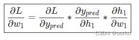
首先,让我们根据以下方法(链式法则)重写偏导数:
![]()
这里![]() 我们可以求得,由于前面的MSE均方误差计算的就是神经网络的误差,MSE作为损失函数,所以有等式:
我们可以求得,由于前面的MSE均方误差计算的就是神经网络的误差,MSE作为损失函数,所以有等式:
![]()
所以可以得出:
![]()
这里使用符合函数求导法则(对于![]() 函数的x进行求导,将得到
函数的x进行求导,将得到![]() ):
):
![]()
![]()
![]()
然后我们再搞清楚![]() ,由于yPred是预测值,而预测值由激活函数输出,所以能够得到等式:
,由于yPred是预测值,而预测值由激活函数输出,所以能够得到等式:
![]()
由于改变w1只对h1有影响,所以可以写成: 
我们再对h1做同样的步骤(h1是上一层的激活函数),![]() ,同样是复合函数求导法则:
,同样是复合函数求导法则:

对于激活函数sigmoid的倒数:

最终整合起来:
这种通过逆向计算偏导数的系统称为反向传播。
推导当前神经网络反向传播所用到的所有偏导公式:
![]()
![]()
![]()
![]()
![]()
![]()
![]()
![]()
![]()
例子:
我们将继续假设数据集中只有 爱丽丝:
| 名字 | 重量(减去 135) | 高度(减去 66) | 性 |
|---|---|---|---|
| 爱丽丝 | -2 | -1 | 1 |
让我们将所有权重初始化为1以及所有偏置为0.如果我们通过网络进行前馈传递,我们会得到:
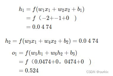
网络输出yPred=0.524,这并不强烈支持男性 或女性 .让我们计算一下![]()

这里用到了上面所求得的sigmoid的倒数。
我们成功了!这告诉我们,由于![]() 所求的偏导结果为0.0214,是个正数,函数单调递增,所以
所求的偏导结果为0.0214,是个正数,函数单调递增,所以
如果我们要增加w1(权重),L(损失)结果会增大一点点。
训练:随机梯度下降
我们现在拥有训练神经网络所需的所有工具!我们将使用一种称为随机梯度下降 (SGD) 的优化算法,该算法告诉我们如何改变权重和偏差以最小化损失。
就是这个方程式:
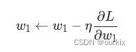
η是一个称为学习率的常数,它控制着我们训练的速度。我们所做的只是用旧权重减去学习率*偏导值:
- 如果
 的值为正数,w1的减少,会使得L减少。
 - 如果的值为负数,w1的增加,会使得L减少。
如果我们对网络中的每个权重和偏差都这样做,损失将慢慢减少,我们的网络将得到改善。
我们的训练过程将如下所示:
- 从我们的数据集中选择一个样本。这就是它随机梯度下降的原因——我们一次只对一个样本进行操作。
- 计算所有损失相对于权重或偏差的偏导数(例如,
 等)。
等)。 - 使用更新公式更新每个权重和偏差。
- 返回步骤 1。
让我们看看它的实际效果吧!
代码:一个完整的神经网络
终于到了实现一个完整的神经网络的时候了:
| 名字 | 重量(减去 135) | 高度(减去 66) | 性 |
|---|---|---|---|
| 爱丽丝 | -2 | -1 | 1 |
| 鲍勃 | 25 | 6 | 0 |
| 查理 | 17 | 4 | 0 |
| 黛安娜 | -15 | -6 | 1 |
import numpy as np

def sigmoid(x):
  # Sigmoid activation function: f(x) = 1 / (1 + e^(-x))
  return 1 / (1 + np.exp(-x))

def deriv_sigmoid(x):
  # Derivative of sigmoid: f'(x) = f(x) * (1 - f(x))
  fx = sigmoid(x)
  return fx * (1 - fx)

def mse_loss(y_true, y_pred):
  # y_true and y_pred are numpy arrays of the same length.
  return ((y_true - y_pred) ** 2).mean()

class OurNeuralNetwork:
  '''
  A neural network with:
    - 2 inputs
    - a hidden layer with 2 neurons (h1, h2)
    - an output layer with 1 neuron (o1)

  *** DISCLAIMER ***:
  The code below is intended to be simple and educational, NOT optimal.
  Real neural net code looks nothing like this. DO NOT use this code.
  Instead, read/run it to understand how this specific network works.
  '''
  def __init__(self):
    # Weights
    self.w1 = np.random.normal()
    self.w2 = np.random.normal()
    self.w3 = np.random.normal()
    self.w4 = np.random.normal()
    self.w5 = np.random.normal()
    self.w6 = np.random.normal()

    # Biases
    self.b1 = np.random.normal()
    self.b2 = np.random.normal()
    self.b3 = np.random.normal()

  def feedforward(self, x):
    # x is a numpy array with 2 elements.
    h1 = sigmoid(self.w1 * x[0] + self.w2 * x[1] + self.b1)
    h2 = sigmoid(self.w3 * x[0] + self.w4 * x[1] + self.b2)
    o1 = sigmoid(self.w5 * h1 + self.w6 * h2 + self.b3)
    return o1

  def train(self, data, all_y_trues):
    '''
    - data is a (n x 2) numpy array, n = # of samples in the dataset.
    - all_y_trues is a numpy array with n elements.
      Elements in all_y_trues correspond to those in data.
    '''
    learn_rate = 0.1
    epochs = 1000 # number of times to loop through the entire dataset

    for epoch in range(epochs):
      for x, y_true in zip(data, all_y_trues):
        # --- Do a feedforward (we'll need these values later)
        sum_h1 = self.w1 * x[0] + self.w2 * x[1] + self.b1
        h1 = sigmoid(sum_h1)

        sum_h2 = self.w3 * x[0] + self.w4 * x[1] + self.b2
        h2 = sigmoid(sum_h2)

        sum_o1 = self.w5 * h1 + self.w6 * h2 + self.b3
        o1 = sigmoid(sum_o1)
        y_pred = o1

        # --- Calculate partial derivatives.
        # --- Naming: d_L_d_w1 represents "partial L / partial w1"
        d_L_d_ypred = -2 * (y_true - y_pred)

        # Neuron o1
        d_ypred_d_w5 = h1 * deriv_sigmoid(sum_o1)
        d_ypred_d_w6 = h2 * deriv_sigmoid(sum_o1)
        d_ypred_d_b3 = deriv_sigmoid(sum_o1)

        d_ypred_d_h1 = self.w5 * deriv_sigmoid(sum_o1)
        d_ypred_d_h2 = self.w6 * deriv_sigmoid(sum_o1)

        # Neuron h1
        d_h1_d_w1 = x[0] * deriv_sigmoid(sum_h1)
        d_h1_d_w2 = x[1] * deriv_sigmoid(sum_h1)
        d_h1_d_b1 = deriv_sigmoid(sum_h1)

        # Neuron h2
        d_h2_d_w3 = x[0] * deriv_sigmoid(sum_h2)
        d_h2_d_w4 = x[1] * deriv_sigmoid(sum_h2)
        d_h2_d_b2 = deriv_sigmoid(sum_h2)

        # --- Update weights and biases
        # Neuron h1
        self.w1 -= learn_rate * d_L_d_ypred * d_ypred_d_h1 * d_h1_d_w1
        self.w2 -= learn_rate * d_L_d_ypred * d_ypred_d_h1 * d_h1_d_w2
        self.b1 -= learn_rate * d_L_d_ypred * d_ypred_d_h1 * d_h1_d_b1

        # Neuron h2
        self.w3 -= learn_rate * d_L_d_ypred * d_ypred_d_h2 * d_h2_d_w3
        self.w4 -= learn_rate * d_L_d_ypred * d_ypred_d_h2 * d_h2_d_w4
        self.b2 -= learn_rate * d_L_d_ypred * d_ypred_d_h2 * d_h2_d_b2

        # Neuron o1
        self.w5 -= learn_rate * d_L_d_ypred * d_ypred_d_w5
        self.w6 -= learn_rate * d_L_d_ypred * d_ypred_d_w6
        self.b3 -= learn_rate * d_L_d_ypred * d_ypred_d_b3

      # --- Calculate total loss at the end of each epoch
      if epoch % 10 == 0:
        y_preds = np.apply_along_axis(self.feedforward, 1, data)
        loss = mse_loss(all_y_trues, y_preds)
        print("Epoch %d loss: %.3f" % (epoch, loss))

# Define dataset
data = np.array([
  [-2, -1],  # Alice
  [25, 6],   # Bob
  [17, 4],   # Charlie
  [-15, -6], # Diana
])
all_y_trues = np.array([
  1, # Alice
  0, # Bob
  0, # Charlie
  1, # Diana
])

# Train our neural network!
network = OurNeuralNetwork()
network.train(data, all_y_trues)
随着网络学习,我们的损失稳步减少:
我们现在可以使用网络来预测性别:
# Make some predictions
emily = np.array([-7, -3]) # 128 pounds, 63 inches
frank = np.array([20, 2])  # 155 pounds, 68 inches
print("Emily: %.3f" % network.feedforward(emily)) # 0.951 - F
print("Frank: %.3f" % network.feedforward(frank)) # 0.039 - M