【论文翻译】RetinaFace: Single-stage Dense Face Localisation in the Wild

论文题目：RetinaFace: Single-stage Dense Face Localisation in the Wild
论文来源:RetinaFace: Single-stage Dense Face Localisation in the Wild
翻译人：BDML@CQUT实验室

RetinaFace: Single-stage Dense Face Localisation in the Wild

Jiankang Deng* 1,2,4 Jia Guo* 2 Y uxiang Zhou1 Jinke Yu2 Irene Kotsia3 Stefanos Zafeiriou1,4 1Imperial College London 2InsightFace 3Middlesex University London 4FaceSoft

自然场景下的单阶段密集人脸定位

Jiankang Deng* 1,2,4 Jia Guo* 2 Y uxiang Zhou1 Jinke Yu2 Irene Kotsia3 Stefanos Zafeiriou1,4 1Imperial College London 2InsightFace 3Middlesex University London 4FaceSoft

Abstract

Though tremendous strides have been made in uncontrolled face detection, accurate and efficient face localisation in the wild remains an open challenge. This paper presents a robust single-stage face detector, named RetinaFace, which performs pixel-wise face localisation on various scales of faces by taking advantages of joint extra-supervised and self-supervised multi-task learning. Specifically, We make contributions in the following five aspects: (1) We manually annotate five facial landmarks on the WIDER FACE dataset and observe significant improvement in hard face detection with the assistance of this extra supervision signal. (2) We further add a self supervised mesh decoder branch for predicting a pixel-wise 3D shape face information in parallel with the existing supervised branches. (3) On the WIDER FACE hard test set, RetinaFace outperforms the state of the art average precision (AP) by 1.1% (achieving AP equal to 91.4%). (4) On the IJB-C test set, RetinaFace enables state of the art methods (ArcFace) to improve their results in face verification (TAR=89.59% for FAR=1e-6). (5) By employing light-weight backbone networks, RetinaFace can run real-time on a single CPU core for a VGA-resolution image. Extra annotations and code have been made available at: https://github.com/deepinsight/ insightface/tree/master/RetinaFace.

摘要

尽管在不受控制的人脸检测方面已经取得了巨大的进步，但在自然环境下精确和高效的人脸定位仍然是一个公开的挑战。本文提出了一种鲁棒的单级人脸检测器，名为RetinaFace，它利用联合的额外监督和自监督多任务学习，在不同尺度的人脸上进行像素化的人脸定位。具体而言，我们在以下五个方面做出了贡献:

(1)在WIDER FACE数据集上手工标注了五个面部标志，并观察到在这种额外的监督信号的帮助下，人脸检测有了显著的改善。
(2) 添加了一个自监督网格编码分支，用于预测一个逐像素的3D人脸信息。该分支与已存在的监督分支并行。
(3)在WIDER FACE测试集上，RetinaFace的平均精度(AP)比目前的平均精度(AP)高出1.1% (AP = 91.4%)。
(4) 在IJB-C测试集上，RetinaFace使当前最好的ArcFace在人脸认证（face verification）上进一步提升（TAR=89.59 FAR=1e-6）。
(5)通过采用轻量级骨干网，RetinaFace可以在单核CPU下实时运行VGA分辨率的图像。

1.Introduction

Automatic face localisation is the prerequisite step of facial image analysis for many applications such as facial attribute (e.g. expression [64] and age [38]) and facial identity recognition [45, 31, 55, 11]. A narrow definition of face localisation may refer to traditional face detection [53, 62], which aims at estimating the face bounding boxes without any scale and position prior. Nevertheless, in this paper we refer to a broader definition of face localisation which includes face detection [39], face alignment [13], pixelwise face parsing [48] and 3D dense correspondence regression [2, 12]. That kind of dense face localisation provides accurate facial position information for all different scales.

Inspired by generic object detection methods [16, 43, 30, 41, 42, 28, 29], which embraced all the recent advances in deep learning, face detection has recently achieved remarkable progress [23, 36, 68, 8, 49]. Different from generic object detection, face detection features smaller ratio variations (from 1:1 to 1:1.5) but much larger scale variations (from several pixels to thousand pixels). The most recent state-of-the-art methods [36, 68, 49] focus on singlestage [30, 29] design which densely samples face locations and scales on feature pyramids [28], demonstrating promising performance and yielding faster speed compared to twostage methods [43, 63, 8]. Following this route, we improve the single-stage face detection framework and propose a state-of-the-art dense face localisation method by exploiting multi-task losses coming from strongly supervised and self-supervised signals. Our idea is examplified in Fig. 1.

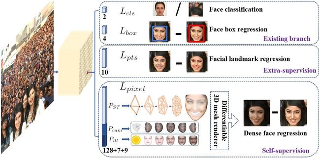
Typically, face detection training process contains both classification and box regression losses [16]. Chen et al. [6] proposed to combine face detection and alignment in a joint cascade framework based on the observation that aligned face shapes provide better features for face classification. Inspired by [6], MTCNN [66] and STN [5] simultaneously detected faces and five facial landmarks. Due to training data limitation, JDA [6], MTCNN [66] and STN [5] have not verified whether tiny face detection can benefit from the extra supervision of five facial landmarks. One of the questions we aim at answering in this paper is whether we can push forward the current best performance (90.3% [67]) on the WIDER FACE hard test set [60] by using extra supervision signal built of five facial landmarks.

In Mask R-CNN [20], the detection performance is significantly improved by adding a branch for predicting an object mask in parallel with the existing branch for bounding box recognition and regression. That confirms that dense pixel-wise annotations are also beneficial to improve detection. Unfortunately, for the challenging faces of WIDER FACE it is not possible to conduct dense face annotation (either in the form of more landmarks or semantic segments). Since supervised signals cannot be easily obtained, the question is whether we can apply unsupervised methods to further improve face detection.

In FAN [56], an anchor-level attention map is proposed to improve the occluded face detection. Nevertheless, the proposed attention map is quite coarse and does not contain semantic information. Recently, self-supervised 3D morphable models [14, 51, 52, 70] have achieved promising 3D face modelling in-the-wild. Especially, Mesh Decoder [70] achieves over real-time speed by exploiting graph convolutions [10, 40] on joint shape and texture. However, the main challenges of applying mesh decoder [70] into the single-stage detector are: (1) camera parameters are hard to estimate accurately, and (2) the joint latent shape and texture representation is predicted from a single feature vector (1 × 1 Conv on feature pyramid) instead of the RoI pooled feature, which indicates the risk of feature shift. In this paper, we employ a mesh decoder [70] branch through self-supervision learning for predicting a pixel-wise 3D face shape in parallel with the existing supervised branches. To summarise, our key contributions are:
• Based on a single-stage design, we propose a novel pixel-wise face localisation method named RetinaFace, which employs a multi-task learning strategy to simultaneously predict face score, face box, five facial landmarks, and 3D position and correspondence of each facial pixel.
• On the WIDER FACE hard subset, RetinaFace outperforms the AP of the state of the art two-stage method (ISRN [67]) by 1.1% (AP equal to 91.4%).
• On the IJB-C dataset, RetinaFace helps to improve ArcFace’s [11] verification accuracy (with TAR equal to 89.59% when FAR=1e-6). This indicates that better face localisation can significantly improve face recognition.
• By employing light-weight backbone networks, RetinaFace can run real-time on a single CPU core for a VGA-resolution image.
• Extra annotations and code have been released to facilitate future research.

1.引言

自动人脸定位是人脸图像分析如人脸属性（表情，年龄，ID识别）的先决步骤。人脸检测传统上的窄定义：在没有任何尺度核位置信息的情况下估计人脸检测框。然而，本文引用了更广泛的人脸定位定义，包括人脸检测、人脸比对、像素化人脸解析和3D密集对应回归。这种密集的面部定位为所有不同的尺度提供了精确的面部位置信息。
受深度学习最新检测方法的启发，这些方人脸检测最近取得了显著进展。与一般的对象检测不同，人脸检测特征比例变化更小(从1:1到1:1.5)，但范围变化更大(从几个像素到1000像素)。，目前最先进的方法集中在单阶段设计上，相比两级级联方法，这种设计获得了不错的性能和速度提升。依据这种路线，我们提升的单级人脸检测框架，并且通过利用强监督和自监督型号的多任务损失，提出了当前最好的密集人脸定位方法。思想如图1：

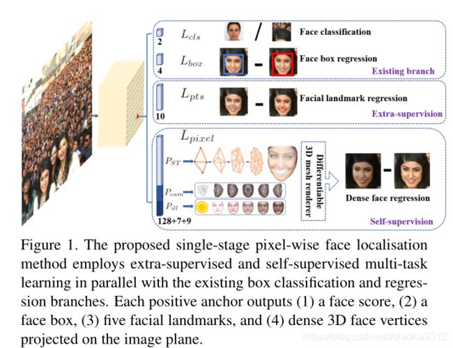
典型的人脸检测训练过程包括分类损失和框回归损失。Chen等人在观察到对齐后的人脸形状能够提供更好的人脸分类特征的基础上，提出将人脸检测与对齐在联合级联框架中结合。基于这种思想，MTCNN和STN同时检测人脸和5个面部关键点。由于训练数据的限制，JDA、MTCNN和STN没有验证小的人脸检测是否可以从五个面部特征点的额外监督中获益。本文中想要回答的一个问题是，是否可以通过使用五个面部关键点构建的额外监督信号来推动当前在WIDER FACE 难测试集上的最佳性能(90.3%)提升。
在 Mask R-CNN中，通过在已有的分支进行边界框识别和回归的同时增加预测对象掩模的分支，检测性能得到了显著提高。这证实了密集的像素级标注也有利于提高检测。但是，对于WIDER FACE具有挑战性的面部，不可能进行密集的面部注释(以更多标注或语义片段的形式)。由于有监督的信号不易获得，我们是否可以使用无监督的方法来进一步改进人脸检测还是一个问题。
FAN提出了一种anchor级别的注意图来改善遮挡人脸的检测。然而，所提出的注意力图非常粗糙，且不包含语义信息。不过最近，自监督的3D 形变模型已经实现了不错的自然环境下三维人脸建模。特别是网格解码器通过在形状和纹理上利用图卷积来实现实时速度。然而,将网格解码器应用到单阶段的结构中的挑战有:(1)相机参数难以准确估计(2) 联合潜在形状和纹理是单一的特征向量中预测的(特征金字塔上的1×1 Conv)，而不是ROI池化特征，这会有特征转移的风险。在本文中，我们使用了一个通过自监督学习的网格解码器分支，用于与现有的监督分支并行地预测像素级的3D人脸形状。总的来说我们的主要贡献如下：
==
• 在单阶段设计的基础上，提出了一种名为RetinaFace的基于像素的人脸定位方法，该方法采用多任务学习策略来同时预测人脸评分、人脸框、五个人脸关键点以及每个人脸像素的三维位置和对应关系。
• 在WIDER FACE hard子集上，RetinaFace比当前的两阶段方法高出了1.1%（平均精度达到91.4%）
• 在IJB-C数据集上，RetinaFace有助于提高ArcFace的验证精度(TAR =89.59% 、FAR=1e-6)。这表明更好的人脸定位可以显著提高人脸识别能力。
• 通过采用轻量级骨干网，RetinaFace可以在单一CPU核心上实时运行vga分辨率的图像。
• 已经发布额外的注释和代码，以促进未来的研究。==

2.Related work

Image pyramid v.s. feature pyramid:
The sliding-window paradigm, in which a classifier is applied on a dense image grid, can be traced back to past decades. The milestone work of Viola-Jones [53] explored cascade chain to reject false face regions from an image pyramid with real-time efficiency, leading to the widespread adoption of such scale-invariant face detection framework [66, 5]. Even though the sliding-window on image pyramid was the leading detection paradigm [19, 32], with the emergence of feature pyramid [28], sliding-anchor [43] on multi-scale feature maps [68, 49], quickly dominated face detection.

Two-stage v.s. single-stage:
Current face detection methods have inherited some achievements from generic object detection approaches and can be divided into two categories: two-stage methods (e.g. Faster R-CNN [43, 63, 72]) and single-stage methods (e.g. SSD [30, 68] and RetinaNet [29, 49]). Two-stage methods employed a “proposal and refinement” mechanism featuring high localisation accuracy. By contrast, single-stage methods densely sampled face locations and scales, which resulted in extremely unbalanced positive and negative samples during training. To handle this imbalance, sampling [47] and re-weighting [29] methods were widely adopted. Compared to two-stage methods, single-stage methods are more efficient and have higher recall rate but at the risk of achieving a higher false positive rate and compromising the localisation accuracy.

Context Modelling
To enhance the model’s contextual reasoning power for capturing tiny faces [23], SSH [36] and PyramidBox [49] applied context modules on feature pyramids to enlarge the receptive field from Euclidean grids. To enhance the non-rigid transformation modelling capacity of CNNs, deformable convolution network (DCN) [9, 74] employed a novel deformable layer to model geometric transformations. The champion solution of the WIDER Face Challenge 2018 [33] indicates that rigid (expansion) and non-rigid (deformation) context modelling are complementary and orthogonal to improve the performance of face detection.

Multi-task Learning:
Joint face detection and alignment is widely used [6, 66, 5] as aligned face shapes provide better features for face classification. In Mask R-CNN [20],the detection performance was significantly improved by adding a branch for predicting an object mask in parallel with the existing branches. Densepose [1] adopted the architecture of Mask-RCNN to obtain dense part labels and coordinates within each of the selected regions. Nevertheless, the dense regression branch in [20, 1] was trained by supervised learning. In addition, the dense branch was a small FCN applied to each RoI to predict a pixel-to-pixel dense mapping.

2.相关工作

图像金字塔vs特征金字塔:
最早的滑动窗口可以追溯到几十年前（即将分类器应用在一个密集的图像网格中）。Viola-Jones的里程碑式工作探索了级联链，可以实时高效地从图像金字塔中剔除虚假的人脸区域，这种尺度不变的人脸检测框架开始被广泛采用。虽然图像金字塔上的滑动窗口是主要的检测范式，但随着特征金字塔的出现，多尺度特征图上的滑动锚点迅速占据了人脸检测的主导地位。
两阶段vs .单阶段:
目前的人脸检测方法继承了一般目标检测方法的一些成果，可以分为两类:两阶段方法(如FAST R-CNN)和单阶段方法(如SSD和RetinaNet)。两阶段的方法采用了“proposal and refinement”机制，具有很高的定位精度。而单阶段法密集采样人脸位置和尺度，导致训练过程中正样本和负样本极不平衡。为了处理这种不平衡，广泛采用了采样和re-weighting的方法。与两阶段法相比，单阶段法效率更高，召回率更高，但存在假阳性率更高、定位准确性下降的风险。
上下文建模:
为了增强模型捕捉小人脸时的上下文推理能力，SSH和PyramidBox在特征金字塔上应用上下文模块来扩大欧几里得网格中获取的感受野。为了增强CNNs的非刚性变换建模能力，可变形卷积网络(DCN)采用了一种新的可变形层来建模几何变换。2018年的WIDER Face Challenge的冠军解决方案表明，刚性(扩展)和非刚性(变形)上下文建模是互补和正交的，可以提高人脸检测的性能。
多任务学习:
人脸检测与对齐的结合被广泛应用，因为对齐后的人脸形状为人脸分类提供了更好的特征。在Mask R-CNN中，通过在已有的分支中并行添加一个预测对象掩码的分支，显著提高了检测性能。Densepose采用了Mask-RCNN的架构，获得每个选定区域内的稠密部分标签和坐标。稠密回归分支是通过监督学习来训练的。此外，密集分支是一个小的FCN应用于每个RoI，以预测像素到像素的密集映射。

3.RetinaFace

3.1. Multi-task Loss
For any training anchor i, we minimise the following multi-task loss:
$$L=L_{cls}\left(p_i,p_i^{\ast }\right)+{\lambda }_1{p}_i^{\ast }{L}_{box}\left(t_i,t_i^{\ast }\right)+{\lambda }_2{p}_i^{\ast }{L}_{pts}\left(l_i,l_i^{\ast }\right)+{\lambda }_3{p}_i^{\ast }{L}_{pixel}$$
(1) Face classification loss$L_{cls}\left(p_i,p_i^{\ast }\right)$ , where $p_i$ is the predicted probability of anchor $i$ being a face and $p_i$ is 1 for the positive anchor and 0 for the negative anchor. The classification loss $L_{cls}$ is the softmax loss for binary classes (face/not face). (2) Face box regression loss $L_{box}\left(t_i,t_i^{\ast }\right)$ , where $t_i={\left\{t_x,t_y,t_w,t_h\right\}}_i$ and $t_i^{\ast }={\left\{t_x^{\ast },t_y^{\ast },t_w^{\ast },t_h^{\ast }\right\}}_i$ resent the coordinates of the predicted box and ground-truth box associated with the positive anchor. We follow [16] to normalise the box regression targets (i.e. centre location, width and height) and use $L_{box}\left(t_i,t_i^{\ast }\right)=R\left(t_i-t_i^{\ast }\right)$ , where R is the robust loss function (smooth-L1) defined in [16]. (3) Facial landmark regression loss $L_{pts}$, where $l_i={\left\{l_{x1},l_{y2},...,l_{x5},l_{y5}\right\}}_i$and represent the predicted five facial landmarks and groundtruth associated with the positive anchor. Similar to the box centre regression, the five facial landmark regression also employs the target normalisation based on the anchor centre. (4) Dense regression loss Lpixel (refer to Eq. 3). The loss-balancing parameters ${\lambda }_1-{\lambda }_3$ are set to 0.25, 0.1 and 0.01, which means that we increase the significance of better box and landmark locations from supervision signals.

3.2. Dense Regression Branch
Mesh Decoder. We directly employ the mesh decoder (mesh convolution and mesh up-sampling) from [70, 40], which is a graph convolution method based on fast localised spectral filtering [10]. In order to achieve further acceleration, we also use a joint shape and texture decoder similarly to the method in [70], contrary to [40] which only decoded shape.

Below we will briefly explain the concept of graph convolutions and outline why they can be used for fast decoding. As illustrated in Fig. 3(a), a 2D convolutional operation is a “kernel-weighted neighbour sum” within the Euclidean grid receptive field. Similarly, graph convolution also employs the same concept as shown in Fig. 3(b). However, the neighbour distance is calculated on the graph by counting the minimum number of edges connecting two vertices. We follow [70] to define a coloured face mesh $G=\left(\nu ,\epsilon \right)$, where $\nu \in {\mathbb{R}}^{n\ast 6}$ is a set of face vertices containing the joint shape and texture information, and$\epsilon \in {\left\{0,1\right\}}^{n\ast n}$ is a sparse adjacency matrix encoding the connection status between vertices. The graph Laplacian is defined as $L=D-\epsilon \in {\mathbb{R}}^{n\ast n}$ where $D\in {\mathbb{R}}^{n\ast n}$ is a diagonal matrix with $D_{ij}={\sum }_j{\epsilon }_{ij}$.

Following [10, 40, 70], the graph convolution with kernel $g_{\theta }$can be formulated as a recursive Chebyshev polynomial truncated at order K,$$y=g_{\theta }{\left(L\right)}_x=\sum _{k=0}^{K-1}{\theta }_k{T}_k{\left(L\right)}_x$$where $\theta \in {\mathbb{R}}^K$ is a vector of Chebyshev coefficients and $T_k\left(L\right)\in {\mathbb{R}}^{n\ast n}$ is the Chebyshev polynomial of order k evaluated at the scaled Laplacian $L$. Denoting $x_k=T_k\left(L\right)x\in {\mathbb{R}}^n$, we can recurrently compute $x_k=2L{x}_{k-1}-x_{k-2}$ with$x_0=x$and$x_1=L_k$ . The whole filtering operation is extremely efficient including $K$ sparse matrix-vector multiplications and one dense matrix-vector multiplication $y=g_{\theta }\left(L\right)x=\left[{\overline{x}}_0,...,{\overline{x}}_{K-1}\right]\theta$.

Differentiable Renderer. After we predict the shape and texture parameters $P_{ST}\in {\mathbb{R}}^{128}$, we employ an efficient differentiable 3D mesh renderer [14] to project a coloured mesh $D_{P_{ST}}$ onto a 2D image plane with camera parameters $P_{cam}=\left[x_c,y_c,z_c,x_c^{{}^{\prime }},y_c^{{}^{\prime }},z_c^{{}^{\prime }},f_c\right]$(i.e. camera location, camera pose and focal length) and illumination parameters
$P_{ill}=\left[x_l,y_l,z_l,r_l,g_l,b_l,r_a,g_a,b_a\right]$ (i.e. location of point light source, colour values and colour of ambient lighting).

Dense Regression Loss. Once we get the rendered 2D face $R\left(D_{P_{ST}},p_{cam},P_{ill}\right)$, we compare the pixel-wise difference of the rendered and the original 2D face using the following function:$$L_{pixel}=\frac{1}{W\ast H}\sum _i^W\sum _j^H\parallel R{\left(D_{P_{ST}},p_{cam},P_{ill}\right)}_{i,j}-I_{i,j}^{\ast }{\parallel }_1$$(3)
where $W$and $H$ are the width and height of the anchor crop$I_{i,j}^{\ast }$respectively.

3.RetinaFace

3.1多任务损失
对于每一个anchor i最小化多任务损失函数
$$L=L_{cls}\left(p_i,p_i^{\ast }\right)+{\lambda }_1{p}_i^{\ast }{L}_{box}\left(t_i,t_i^{\ast }\right)+{\lambda }_2{p}_i^{\ast }{L}_{pts}\left(l_i,l_i^{\ast }\right)+{\lambda }_3{p}_i^{\ast }{L}_{pixel}$$
人脸分类损失$L_{cls}\left(p_i,p_i^{\ast }\right)$ ，其中$p_i$是anchor中是一张脸的概率，当anchor为正例是$p_i^{\ast }$等于1，anchor是负例时等于0。分类损失$L_{cls}$是二分类中的softmax损失（是人脸/非人脸）。(2) 人脸回归框损失 $L_{box}\left(t_i,t_i^{\ast }\right)$，其中$t_i={\left\{t_x,t_y,t_w,t_h\right\}}_i,t_i^{\ast }={\left\{t_x^{\ast },t_y^{\ast },t_w^{\ast },t_h^{\ast }\right\}}_i$ 表示与正样本anchor对应的预测框的位置和真实标注框的位置。归一化box回归目标并使用$L_{box}\left(t_i,t_i^{\ast }\right)=R\left(t_i-t_i^{\ast }\right)$，其中R是smooth—l1鲁棒损失函数。(3)面部关键点回归损失$L_{pts}\left(l_i,l_i^{\ast }\right)$，其中$l_i={\left\{l_{x1},l_{y2},...,l_{x5},l_{y5}\right\}}_i$ 分别表示正样本人脸anchor5关键点的预测和真值。与box回归一致，人脸5个关键点会同样使用目标归一化。(4) 密集回归损失$L_{pixel}$参见公式3。 ${\lambda }_1-{\lambda }_3$的值分别设置为0.25,0.1,0.01，意味着提升了来自监督信号的更好人脸框和五点位置的重要性。

3.2密集回归分支
网格解码器：直接利用网格解码器(网格卷积和网格上采样)，也就是基于快速局部谱滤波器（fast localised spectral filtering）的图卷积方法。为了获得更快的速度，我们联合形状和上下文解码。
下面我们将简要解释图卷积的概念，并概述为什么它们可以用于快速解码。如图3(a)所示，二维卷积操作是欧氏网格感受野内的“近邻核加权求和”。 类似的，图卷积利用了图3（b）中的类似感念。然而，图近邻距离的计算方法是通过连接两个顶点的边的最小数量。定义一个人脸网格$G=\left(\nu ,\epsilon \right)$， $\nu \in {\mathbb{R}}^{n\ast 6}$是人脸顶点集合，包含形状和纹理信息。 $\epsilon \in {\left\{0,1\right\}}^{n\ast n}$是一个稀疏临接矩阵用于编码两个顶点之间的连接状态。图拉普拉斯定义为$L=D-\epsilon \in {\mathbb{R}}^{n\ast n}$其中$D\in {\mathbb{R}}^{n\ast n}$是一个对角矩阵$D_{ij}={\sum }_j{\epsilon }_{ij}$.

核$g_{\theta }$的图卷积可以用切比雪夫K阶多项式展开来表示：
$$y=g_{\theta }{\left(L\right)}_x=\sum _{k=0}^{K-1}{\theta }_k{T}_k{\left(L\right)}_x$$ 其中$\theta \in {\mathbb{R}}^K$为切比雪夫系数向量，$T_k\left(L\right)\in {\mathbb{R}}^{n\ast n}$ 是尺度化的拉普拉斯$L$. 的k阶切比雪夫多项式。$x_k=T_k\left(L\right)x\in {\mathbb{R}}^n$,可以迭代计算$x_k=2L{x}_{k-1}-x_{k-2}$在$x_0=x$,$x_1=L_k$ 。整个计算过程是非常高效的，包括K个稀疏矩阵向量乘法和一个密集的矩阵向量乘法 $y=g_{\theta }\left(L\right)x=\left[{\overline{x}}_0,...,{\overline{x}}_{K-1}\right]\theta$。

可微渲染器：在预测的形状和纹理参数$P_{ST}\in {\mathbb{R}}^{128}$后,采用一种高效的可微的3 d网格渲染器将彩色网格$D_{P_{ST}}$ 投影到2 D图像平面上，利用摄像机参数 $P_{cam}=\left[x_c,y_c,z_c,x_c^{{}^{\prime }},y_c^{{}^{\prime }},z_c^{{}^{\prime }},f_c\right]$ (即摄像头位置,摄像头的形状和焦距)以及照明参数$P_{ill}=\left[x_l,y_l,z_l,r_l,g_l,b_l,r_a,g_a,b_a\right]$ (即点光源的位置、颜色值和环境光颜色)。
密集回归损失：在像素级上比较了渲染器和2D平面上的不同，使用如下公式：
$$L_{pixel}=\frac{1}{W\ast H}\sum _i^W\sum _j^H\parallel R{\left(D_{P_{ST}},p_{cam},P_{ill}\right)}_{i,j}-I_{i,j}^{\ast }{\parallel }_1$$(3)
W、H是anchor区域 $I_{i,j}^{\ast }$的宽和高

4. Experiments

4.1. Dataset
The WIDER FACE dataset [60] consists of 32,203 images and 393,703 face bounding boxes with a high degree of variability in scale, pose, expression, occlusion and illumination. The WIDER FACE dataset is split into training (40%), validation (10%) and testing (50%) subsets by randomly sampling from 61 scene categories. Based on the detection rate of EdgeBox [76], three levels of difficulty (i.e. Easy, Medium and Hard) are defined by incrementally incorporating hard samples.
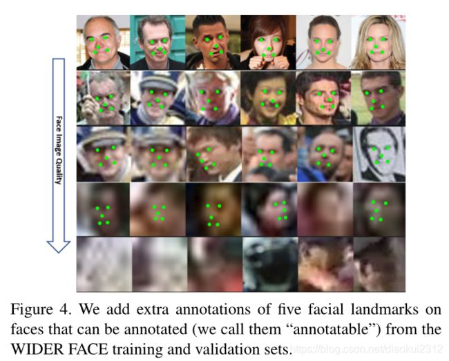
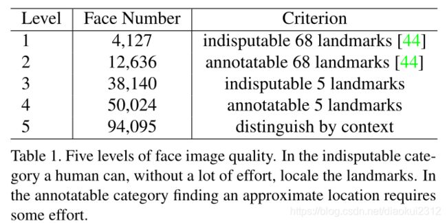
Extra Annotations. As illustrated in Fig. 4 and Tab. 1, we define five levels of face image quality (according to how difficult it is to annotate landmarks on the face) and annotate five facial landmarks (i.e. eye centres, nose tip and mouth corners) on faces that can be annotated from the WIDER FACE training and validation subsets. In total, we have annotated 84.6k faces on the training set and 18.5k faces on the validation set.

Extra Annotations. As illustrated in Fig. 4 and Tab. 1, we
define five levels of face image quality (according to how difficultitis to annotate landmarks on the face)and annotate five facial landmarks (i.e. eye centres, nose tip and mouth corners) on faces that can be annotated from the WIDER FACE training and validation subsets. In total, we have annotated 84.6k faces on the training set and 18.5k faces on the validation set.

4.2. Implementation details
Feature Pyramid. RetinaFace employs feature pyramid levels from P2 to P6, where P2 to P5 are computed from the output of the corresponding ResNet residual stage (C2 through C5) using top-down and lateral connections as in [28, 29]. P6 is calculated through a 3×3 convolution with stride=2 on C5. C1 to C5 is a pre-trained ResNet-152 [21] classification network on the ImageNet-11k dataset while P6 are randomly initialised with the “Xavier” method [17].

Context Module. Inspired by SSH [36] and PyramidBox [49], we also apply independent context modules on five feature pyramid levels to increase the receptive field and enhance the rigid context modelling power. Drawing lessons from the champion of the WIDER Face Challenge 2018 [33], we also replace all 3 × 3 convolution layers within the lateral connections and context modules by the deformable convolution network (DCN) [9, 74], which further strengthens the non-rigid context modelling capacity.

Loss Head. For negative anchors, only classification loss is applied. For positive anchors, the proposed multi-task loss is calculated. We employ a shared loss head (1 × 1 conv) across different feature maps Hn × Wn × 256,n ∈ {2,…,6}. For the mesh decoder, we apply the pre-trained model [70], which is a small computational overhead that allows for efficient inference.

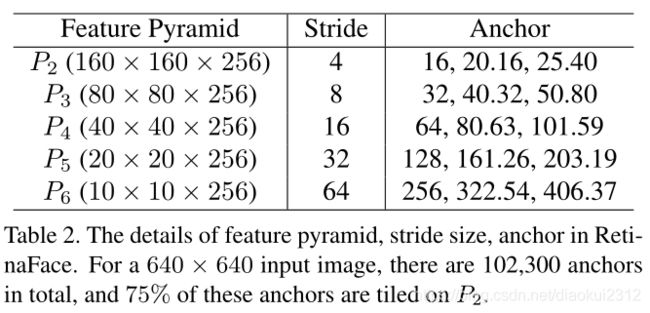
Anchor Settings. As illustrated in Tab. 2, we employ scalespecific anchors on the feature pyramid levels from P2 to P6 like [56]. Here, P2 is designed to capture tiny faces by tiling small anchors at the cost of more computational time and at the risk of more false positives. We set the scale step at 21/3 and the aspect ratio at 1:1. With the input image size at 640 × 640, the anchors can cover scales from 16 × 16 to 406 × 406 on the feature pyramid levels. In total, there are 102,300 anchors, and 75% of these anchors are from P2.

During training, anchors are matched to a ground-truth box when IoU is larger than 0.5, and to the background when IoU is less than 0.3. Unmatched anchors are ignored during training. Since most of the anchors (> 99%) are negative after the matching step, we employ standard OHEM [47, 68] to alleviate significant imbalance between the positive and negative training examples. More specifically, we sort negative anchors by the loss values and select the top ones so that the ratio between the negative and positive samples is at least 3:1.

Data Augmentation. Since there are around 20% tiny faces in the WIDER FACE training set, we follow [68, 49] and randomly crop square patches from the original images and resize these patches into 640 × 640 to generate larger training faces. More specifically, square patches are cropped from the original image with a random size between [0.3, 1] of the short edge of the original image. For the faces on the crop boundary, we keep the overlapped part of the face box if its centre is within the crop patch. Besides random crop, we also augment training data by random horizontal flip with the probability of 0.5 and photo-metric colour distortion [68].

Training Details. We train the RetinaFace using SGD optimiser (momentum at 0.9, weight decay at 0.0005, batch size of 8 × 4) on four NVIDIA Tesla P40 (24GB) GPUs. The learning rate starts from 10−3, rising to 10−2 after 5 epochs, then divided by 10 at 55 and 68 epochs. The training process terminates at 80 epochs.

Testing Details. For testing on WIDER FACE, we follow the standard practices of [36, 68] and employ flip as well as multi-scale (the short edge of image at [500,800,1100,1400,1700]) strategies. Box voting [15] is applied on the union set of predicted face boxes using an IoU threshold at 0.4.

4.3. Ablation Study
To achieve a better understanding of the proposed RetinaFace, we conduct extensive ablation experiments to examine how the annotated five facial landmarks and the proposed dense regression branch quantitatively affect the performance of face detection. Besides the standard evaluation metric of average precision (AP) when IoU=0.5 on the Easy, Medium and Hard subsets, we also make use of the development server (Hard validation subset) of the WIDER Face Challenge 2018 [33], which employs a more strict evaluation metric of mean AP (mAP) for IoU=0.5:0.05:0.95, rewarding more accurate face detectors。

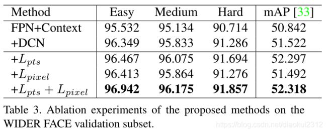
As illustrated in Tab. 3, we evaluate the performance of several different settings on the WIDER FACE validation set and focus on the observations of AP and mAP on the Hard subset. By applying the practices of state-of-the-art techniques (i.e. FPN, context module, and deformable convolution), we set up a strong baseline (91.286%), which is slightly better than ISRN [67] (90.9%). Adding the branch of five facial landmark regression significantly improves the face box AP (0.408%) and mAP (0.775%) on the Hard subset, suggesting that landmark localisation is crucial for improving the accuracy of face detection. By contrast, adding the dense regression branch increases the face box AP on Easy and Medium subsets but slightly deteriorates the results on the Hard subset, indicating the difficulty of dense regression under challenging scenarios. Nevertheless, learning landmark and dense regression jointly enables a further improvement compared to adding landmark regression only. This demonstrates that landmark regression does help dense regression, which in turn boosts face detection performance even further.

4.4. Face box Accuracy
Following the stander evaluation protocol of the WIDER FACE dataset, we only train the model on the training set and test on both the validation and test sets. To obtain the evaluation results on the test set, we submit the detection results to the organisers for evaluation. As shown in Fig. 5, we compare the proposed RetinaFace with other 24 state-of-the-art face detection algorithms (i.e. Multiscale Cascade CNN [60], Two-stage CNN [60], ACFWIDER [58], Faceness-WIDER [59], Multitask Cascade CNN [66], CMS-RCNN [72], LDCF+ [37], HR [23], Face R-CNN [54], ScaleFace [61], SSH [36], SFD [68], Face RFCN [57], MSCNN [4], FAN [56], Zhu et al. [71], Pyramid Box [49], FDNet [63], SRN [8], FANet [65], DSFD [27], DFS [50], VIM-FD [69], ISRN [67]). Our approach out　performs these state-of-the-art methods in terms of AP. More specifically, RetinaFace produces the best AP in all subsets of both validation and test sets, i.e., 96.9% (Easy), 96.1% (Medium) and 91.8% (Hard) for validation set, and 96.3% (Easy), 95.6% (Medium) and 91.4% (Hard) for test set. Compared to the recent best performed method [67], RetinaFace sets up a new impressive record (91.4% v.s. 90.3%) on the Hard subset which contains a large number of tiny faces.

In Fig. 6, we illustrate qualitative results on a selfie with dense faces. RetinaFace successfully finds about 900 faces (threshold at 0.5) out of the reported 1,151 faces. Besides accurate bounding boxes, the five facial landmarks predicted by RetinaFace are also very robust under the variations of pose, occlusion and resolution. Even though there are some failure cases of dense face localisation under heavy occlusion, the dense regression results on some clear and large faces are good and even show expression variations.

4.5. Five Facial Landmark Accuracy
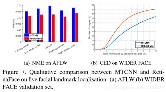
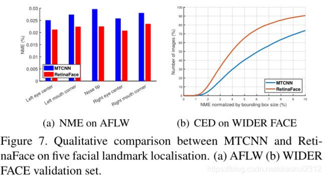
To evaluate the accuracy of five facial landmark localisation, we compare RetinaFace with MTCNN [66] on the AFLW dataset [ ] (24,386 faces) as well as the WIDER FACE validation set (18.5k faces). Here, we employ the (√W × H) face box size ( W × H) as the normalisation distance. As shown in Fig. 7(a), we give the mean error of each facial landmark on the AFLW dataset [73]. RetinaFace significantly decreases the normalised mean errors (NME) from 2.72% to 2.21% when compared to MTCNN. In Fig. 7(b), we show the cumulative error distribution (CED) curves on the WIDER FACE validation set. Compared to MTCNN, RetinaFace significantly decreases the failure rate from２６.31% to 9.37% (the NME threshold at 10%).

４.6. Dense Facial Landmark Accuracy
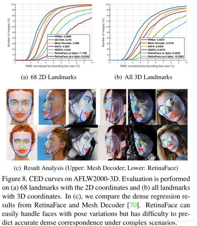
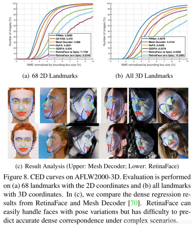
Besides box and five facial landmarks, RetinaFace also outputs dense face correspondence, but the dense regression branch is trained by self-supervised learning only. Following [12, 70], we evaluate the accuracy of dense facial landmark localisation on the AFLW2000-3D dataset [75]considering (1) 68 landmarks with the 2D projection coordinates and (2) all landmarks with 3D coordinates. Here,the mean error is still normalised by the bounding box size [75]. In Fig. 8(a) and 8(b), we give the CED curves of state-of-the-art methods [12, 70, 75, 25, 3] as well as RetinaFace. Even though the performance gap exists between supervised and self-supervised methods, the dense regression results of RetinaFace are comparable with these state-of-the-art methods. More specifically, we observe that(1) five facial landmarks regression can alleviate the training difficulty of dense regression branch and significantly improve the dense regression results. (2) using single-stage features (as in RetinaFace) to predict dense correspondence parameters is much harder than employing (Region of Interest) RoI features (as in Mesh Decoder [70]). As illustrated in Fig. 8©, RetinaFace can easily handle faces with pose variations but has difficulty under complex scenarios. This indicates that mis-aligned and over-compacted feature representation (1 × 1 × 256 in RetinaFace) impedes the single-stage framework achieving high accurate dense regression outputs. Nevertheless, the projected face regions in the dense regression branch still have the effect of attention [56] which can help to improve face detection as confirmed in the section of ablation study.

4.7. Face Recognition Accuracy
Face detection plays a crucial role in robust face recognition but its effect is rarely explicitly measured. In this paper, we demonstrate how our face detection method can boost the performance of a state-of-the-art publicly available face recognition method, i.e. ArcFace [11]. ArcFace [11] studied how different aspects in the training process of a deep convolutional neural network (i.e., choice of the training set, the network and the loss function) affect large scale face recognition performance. However, ArcFace paper did not study the effect of face detection by applying only the MTCNN [66] for detection and alignment. In this paper, we replace MTCNN by RetinaFace to detect and align all of the training data (i.e. MS1M [18]) and test data (i.e. LFW [24], CFP-FP [46], AgeDB-30 [35] and IJBC [34]), and keep the embedding network (i.e. ResNet100 [21]) and the loss function (i.e. additive angular margin) exactly the same as ArcFace.

In Tab1. , we show the influence of face detection and alignment on deep face recognition (i.e. ArcFace) by comparing the widely used MTCNN [66] and the proposed RetinaFace. The results on CFP-FP, demonstrate that RetinaFace can boost ArcFace’s verification accuracy from 98.37% to 99.49%. This result shows that the performance of frontal-profile face verification is now approaching that of frontal-frontal face verification (e.g. 99.86% on LFW).

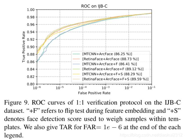
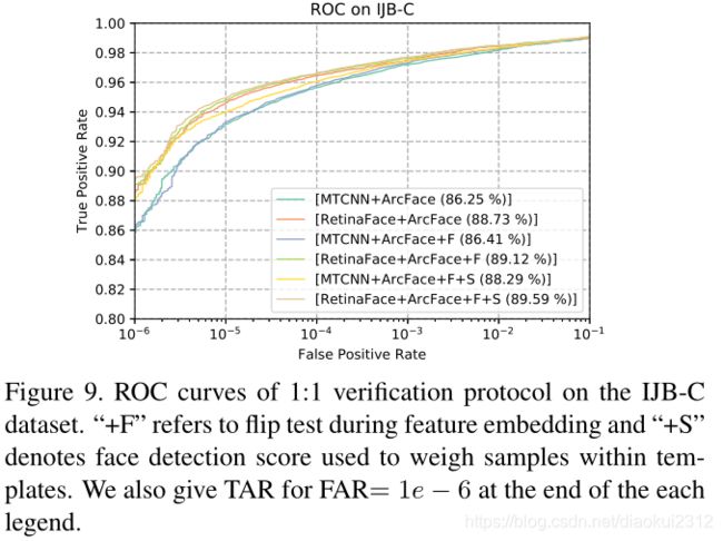
In Fig. 9, we show the ROC curves on the IJB-C dataset as well as the TAR for FAR= 1e − 6 at the end of each legend. We employ two tricks (i.e. flip test and face detection score to weigh samples within templates) to progressively improve the face verification accuracy. Under fair comparison, TAR (at FAR= 1e − 6) significantly improves from 88.29% to 89.59% simply by replacing MTCNN with RetinaFace. This indicates that (1) face detection and alignment significantly affect face recognition performance and (2) RetinaFace is a much stronger baseline that MTCNN for face recognition applications.

4.8. Inference Efficiency
During testing, RetinaFace performs face localisation in a single stage, which is flexible and efficient. Besides the above-explored heavy-weight model (ResNet-152, size of 262MB, and AP 91.8% on the WIDER FACE hard set), we also resort to a light-weight model (MobileNet-0.25 [22], size of 1MB, and AP 78.2% on the WIDER FACE hard set) to accelerate the inference.

For the light-weight model, we can quickly reduce the data size by using a 7 × 7 convolution with stride=4 on the input image, tile dense anchors on P3, P4 and P5 as in [36], and remove deformable layers. In addition, the first two convolutional layers initialised by the ImageNet pre-trained model are fixed to achieve higher accuracy.

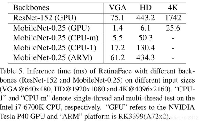
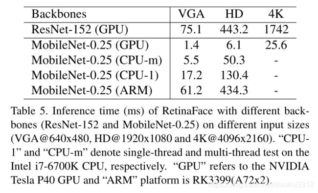
Tab. 5 gives the inference time of two models with respect to different input sizes. We omit the time cost on the dense regression branch, thus the time statistics are irrelevant to the face density of the input image. We take advantage of TVM [7] to accelerate the model inference and timing is performed on the NVIDIA Tesla P40 GPU, Intel i76700K CPU and ARM-RK3399, respectively. RetinaFace ResNet-152 is designed for highly accurate face localisation, running at 13 FPS for VGA images (640 × 480). By contrast, RetinaFace-MobileNet-0.25 is designed for highly efficient face localisation which demonstrates considerable real-time speed of 40 FPS at GPU for 4K images (4096×2160), 20 FPS at multi-thread CPU for HD images (1920 × 1080), and 60 FPS at single-thread CPU for VGA images (640 × 480). Even more impressively, 16 FPS at ARM for VGA images (640×480) allows for a fast system on mobile devices.

4.数据集

4.1 WIDER FACE
WIDER　ＦＡＣＥ数据集包含３２３０３张图像，３９３７０３个人脸框，尺度、姿势、表情、遮挡　和光照变化都很大。并通过从６１个场景中随机抽样，把数据集４０％划分为训练集，１０％作为验证集，５０％作为测试集。基于对ＥｄｇｅＢｏｘ的检测率，通过递增合并难样本，分为三个等级简单、中等、困难。
额外标注：如图４和表１所示，我们定义了五个等级的人脸质量级别（依据人脸标记的难度）并在WIDER　FACE的训练子集和测试子集上标注了五个面部关键点（眼睛中间、鼻尖、嘴角）。我们在训练集标记了８４.６ｋ个人脸，在测试集上标记了１８.５ｋ人脸。

特征金字塔：RetinaFace采用P2到P6的特征层，其中P2- p5是使用自上而下和横向连接从相应ResNet残差阶段(C2到C5)的输出中计算出来的。P6是在C5的基础上，使用3*3，stride=2的卷积计算出来的。C1-C5是ResNet-152分类网络在ImageNet-11k数据集上预训练出来的。P6是用Xavier方法随机出的。
上下文模块：受SSH和pyramibox的启发，我们还在五个特征金字塔上应用了独立的上下文模块，以增加感受野，增强刚性上下文建模能力。借鉴2018年WIDER Face挑战赛的冠军，我们还用可变形卷积网络（DCN）替换了横向连接和上下文模块中的所有3×3卷积层，这进一步增强了非刚性上下文建模能力。
损失头：对于负例，仅应用分类损失。对于正例，计算了所提出的多任务损失。我们在不同的特征映射中使用了一个共享的损失头（1×1 conv）Hn × Wn × 256,n ∈ {2,…,6}.。对于网格解码器，采用预先训练的模型，这是一个小的计算开销，允许有效的推理。
Anchor设定：如表2所示，我们在P2到P6的特征金字塔层次上使用特定比例的anchor。P2设定的anchor比较小用来捕捉小人脸，但同时计算时间和误报风险也提高了。我们将比例步长设置为21/3，长宽比设置为1:1。当输入图像尺寸为640×640时，anchor可以覆盖16×16到406×406的特征金字塔。总共有102300个anchor，其中75%来自P2。

在训练过程中，当IoU大于0.5时，anchor与ground truth匹配，IoU小于0.3时anchor与背景匹配。训练期间，不匹配的anchor会被忽略。由于匹配步骤后大多数ancho为负例（99%），因此我们采用标准的OHEM来减轻正负训练样本之间显著的不平衡。更具体地说，我们根据损失值对负样本进行排序，并选择最上面的anchor，以便正负样本之间的比率至少为3:1。
数据扩充：由于在WIDER　FACE训练集中大约有20%的小人脸，我们从原始图像中随机裁剪出方形图片区域，并将这些图片调整为640×640，以生成更大的训练人脸数据。具体来说，从原始图像裁剪方形图片，其大小在原始图像短边的[0.3，1]之间。对于裁剪边界上的人脸，如果人脸框的中心在裁剪块内，则保留人脸框的重叠部分。除了随机裁剪外，我们还通过随机水平翻转（概率为0.5）和光度量颜色失真来增加训练数据。
训练细节：我们使用SGD优化器（动量为0.9，权重衰减为0.0005，batch size ＝8×4）在四个NVIDIA Tesla P40（24GB）GPU上训练。学习率从10-3开始，5个世代后上升到10-2，然后在55和68个世代除以10。训练过程在80个世代结束。
测试细节：在ＷＩＤＥＲ　ＦＡＣＥ上测试，利用翻转和多尺度策略（图像的短边为[500、800、1100、1400、1700]）。预测的人脸框集合使用投票策略，阈值设置为０.４
4.3消融实验
为了更好地理解所提出的ＲｅｔｉｎａＦａｃｅ，我们进行了大量的消融实验来研究标注的五个面部关键点和提出的稠密回归分支是如何定量地影响人脸检测性能的。除了使用在简单、中等和困难子集，IoU=0.5时的平均精度（AP）标准评估指标外，我们还利用了2018　WIDER Face挑战的难验证子集，在IoU=0.5:0.05:0.95，测试更严格的AP 。
如表３所示。在WIDER FACE验证集上评价了几种不同设置的性能，并重点研究了困难集上的AP和mAP。通过应用最新技术，FPN、上下文模块和可变形卷积，我们建立了一个较好的baseline（91.286%），略优于ISRN（90.9%）。在困难集上加入五个人脸关键点回归的分支显著提高了人脸检测框的 AP（0.408%）和mAP（0.775%），说明关键点定位对于提高人脸检测的准确性至关重要。相比之下，增加稠密回归分支会增加简单和中等子集上的人脸框 AP，但在困难子集上的结果略有降低，这表明在挑战性场景下密集回归比较困难。尽管如此，在同时添加面部关键点和密集回归分支，比只添加面部关键点结果更好，进一步证明了密集回归分支有助于提高性能。

4.4人脸框准确率
根据WIDER FACE数据集的标准评估协议，我们用训练集训练模型，并在验证集和测试集上进行测试。我们将检测结果提交给组织者进行评估得到测试集评估结果。如图5所示，我们将提出的RetinaFace与其他24种较好的人脸检测算法进行比较。我们的方法在AP方面优于这些较好的方法。具体来说，RetinaFace在所有验证集和测试集ＡＰ最好，即验证集为96.9%（容易）、96.1%（中等）和91.8%（困难），测试集为96.3%（容易）、95.6%（中等）和91.4%（困难）。与目前最好的方法相比，RetinaFace在包含大量小脸的困难子集上创造了一个新的记录（91.4%vs.90.3%）。

如图6，我们展示了一张脸密集的自拍照片的定性结果。图片中共有1151个人脸，RetinaFace成功地找到了900个人脸（阈值为0.5）。除了精确的边界框外，由RetinaFace预测出的五个面部关键点在姿态、遮挡和分辨率变化下也具有很强的鲁棒性。在重度遮挡下，密集人脸定位有失败的案例，但在一些清晰的大人脸上，稠密回归结果良好，甚至可以看到表情变化。

4.5五个人脸关键点准确率
为了评估五个面部关键点定位的准确性，我们在AFLW数据集（24386个人脸）以及WIDER FAE验证集（18.5k个人脸）上比较RetinaFace与MTCNN的效果。（√W×H）作为人脸框归一化距离。如图7（a）所示，给出了AFLW数据集上每个面部关键点的平均误差。与MTCNN相比，RetinaFace使标准化平均误差（NME）从2.72%降低到2.21%。在图7（b）中，我们展示了在WTDER FACE验证集上的累积误差分布（CED）曲线。与MTCNN相比，RetinaFace可显著降低失败率，从26.31%降至9.37%（NME阈值为10%）。

4.6密集人脸关键点准确率
除了box和五个面部关键点外，RetinaFace还输出密集的人脸对应，但密集回归分支仅通过自监督学习进行训练。之后我们评估了AFLW2000-3D数据集上密集面部关键点定位的准确性，（1）2D投影下的68人脸关键点（2）所有关键点的3D坐标。平均误差仍然由边界框大小进行归一化。图8a和图8b是当前最好方法的CED曲线。尽管自监督和有监督方法的性能差异还比较大，但是RetinaFace相比较而言是最好的方法。具体的，我们观察到（1）五个面部关键点回归可以减轻密集回归分支的训练难度，显著提高密集回归结果。（2） 使用单阶段特征（如RetinaFace）预测密集对应参数比使用（感兴趣区域）RoI特征（如Mesh解码器）困难。如图8（c）所示，RetinaFace可以很容易地处理具有姿势变化的面部，但在复杂场景下还有困难。这表明，错误对齐和过度压缩的特征表示（RetinaFace为1×1×256）阻碍了单阶段结构实现高精度的稠密回归输出。尽管如此，回归分支中投影出来的回归区域依然有助于人类检测结果的提升。

4.7人脸识别准确率
人脸检测在鲁棒人脸识别中起着至关重要的作用，但其效果却很少得到明确的衡量。在本文中，演示了我们的人脸检测方法如何提高最先进的公开人脸识别方法ArcFace的性能。ArcFace研究了深度卷积神经网络训练过程中的不同方面（即训练集、网络和损失函数的选择）对大规模人脸识别性能的影响。然而，ArcFace论文并没有研究应用MTCNN进行检测和对齐的人脸检测效果的影响。在本文中，我们用RetinaFace代替MTCNN来检测和校准所有的训练数据（MS1M）和测试数据（LFW、CFP-FP、AgeDB-30、IJBC）,保留原Arcface中使用的Resnet100基础网络以及损失函数.
在表4,通过比较MTCNN和本文提出的RetinaFace算法，说明了人脸检测和对齐,对深度人脸识别的影响。在CFP-FP上的实验结果表明，RetinaFace可以将ArcFace的验证精度从98.37%提高到99.49%。结果表明，目前正面轮廓人脸验证的性能已接近正面人脸验证的性能（如LFW上的99.86%）。

图9，展示了IJB-C数据集上的ROC曲线以及FAR=1e−6的TAR在每个图例的末尾。我们使用两个tricks（翻转测试和人脸检测分数来衡量模板中的样本），以逐步提高人脸验证的准确性。使用retinaface代替mtcnn，TAR从88.29%提升到了89.59%。这表示（1）人脸检测和对齐对人脸识别影响很大（2）Retinaface相比MTCNN更加强壮。

表格5给出了两个模型在不同输入规模下的预测时间。我们忽略了密集回归分支的时间开销，因此时间统计与输入图像的人脸密度无关。利用TVM加速模型，并分别在NVIDIA Tesla P40 GPU、Intel i76700K CPU和ARM-RK3399上进行了计时。RetinaFace ResNet-152是为高度精确的面部定位而设计的，对于VGA图像（640×480），运行速度为13 FPS。相比之下，RetinaFace-MobileNet-0.25是为高效的面部定位而设计的，在GPU上，4K图像（4096×2160）的实时速度是40fps，高清图像的多线程CPU速度是20fps（1920×1080），VGA图像（640×480）的单线程CPU速度是60fps。

5. Conclusions

We studied the challenging problem of simultaneous dense localisation and alignment of faces of arbitrary scales in images and we proposed the first, to the best of our knowledge, one-stage solution (RetinaFace). Our solution outperforms state of the art methods in the current most challenging benchmarks for face detection. Furthermore, when RetinaFace is combined with state-of-the-art practices for face recognition it obviously improves the accuracy. The data and models have been provided publicly available to facilitate further research on the topic.

5.结论

我们研究了图像中任意比例的人脸同时密集定位和对齐这一具有挑战性的问题，并提出了单级解决方案（RetinaFace）。并在当前最具挑战性的人脸检测基准测试中有最好的检测效果。此外，当RetinaFace与最新的人脸识别实践相结合时，它明显地提高了准确性。这些数据和模型已经公开提供，以促进对这一主题的进一步研究。

6. Acknowledgements

Jiankang Deng acknowledges financial support from the Imperial President’s PhD Scholarship and GPU donations from NVIDIA. Stefanos Zafeiriou acknowledges support from EPSRC Fellowship DEFORM (EP/S010203/1), FACER2VM (EP/N007743/1) and a Google Faculty Fellowship.

7.参考文献

References