Shape-Aware Meta-Learning 在模型泛化中引入形状约束
论文来源:Liu, Quande, Qi Dou, and Pheng-Ann Heng. “Shape-aware Meta-learning for Generalizing Prostate MRI Segmentation to Unseen Domains.” In International Conference on Medical Image Computing and Computer-Assisted Intervention, pp. 475-485. Springer, Cham, 2020. (Code from https://github.com/liuquande/SAML)
Motivation
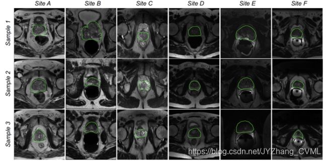
域泛化问题
例如不同中心采集的MRI前列腺数据,存在明显的域差异问题。因此采用在已知中心 (如 Site A, B, C, D, E) 上训练的模型在未知中心 (如 Site F) 上测试,会导致显著的分割错误 —— 即域泛化问题。
元学习 Meta-learning
Meta learning (元学习) 可以用来处理上述模型方法,通过在训练过程中切分数据 meta-train 和 meta-test 来显式模拟已知和未知域之间的域差异。然而此类方法大多数用来处理 image-level 的自然图像分类问题,不适合用来处理逐像素预测的分割问题——其中重要的问题在于如何引入 Shape-based regularization,导致不完整的形状以及含糊的边界。
Shape-Aware Meta-Learning
shape-aware loss function
基于上述对元学习缺点的分析,我们希望模型能够保持形状完整性 shape compactness 和 形状平滑性 shape smoothness。因此,将两个互补的形状约束项引入传统的 meta-learning 损失函数中:
L meta = L seg + λ 1 L compact + λ 2 L smooth \mathcal{L}_{\text {meta}}=\mathcal{L}_{\text {seg}}+\lambda_{1} \mathcal{L}_{\text {compact}}+\lambda_{2} \mathcal{L}_{\text {smooth}} Lmeta=Lseg+λ1Lcompact+λ2Lsmooth
其中 λ 1 \lambda_1 λ1 和 λ 2 \lambda_2 λ2 分别表示对形状完整性和形状平滑性的均衡。
shape complementation
考虑到前列腺呈现 compact shape,因此采用 Iso-Perimetric Quotient 度量 C I P Q = 4 π A / P 2 C_{I P Q}=4 \pi A / P^{2} CIPQ=4πA/P2,其中 A A A 和 P P P 分别代表形状面积和边缘长度。将上述度量转化到分割任务中,形成 shape compactness constraint:
L compact = P 2 4 π A = ∑ i ∈ Ω ( ∇ p u i ) 2 + ( ∇ p v i ) 2 + ϵ 4 π ( ∑ i ∈ Ω ∣ p i ∣ + ϵ ) \mathcal{L}_{\text {compact}}=\frac{P^{2}}{4 \pi A}=\frac{\sum_{i \in \Omega} \sqrt{\left(\nabla p_{u_{i}}\right)^{2}+\left(\nabla p_{v_{i}}\right)^{2}+\epsilon}}{4 \pi\left(\sum_{i \in \Omega}\left|p_{i}\right|+\epsilon\right)} Lcompact=4πAP2=4π(∑i∈Ω∣pi∣+ϵ)∑i∈Ω(∇pui)2+(∇pvi)2+ϵ
直观来说,最小化上述 L c o m p a c t \mathcal{L}_{compact} Lcompact 鼓励分割结果具有完整 compact shape —— 因为不完整的形状常具有较小的区域 A A A 然而具有较大的 P P P,即较大的 L c o m p a c t \mathcal{L}_{compact} Lcompact。
shape smoothness
要求分割结果具有平滑的边缘,通过正则化 domain-invariant contour-relevant background-relevant embedding,提升类内一致性和类间差异性。具体来说,通过 mask-average pooling 方法得到边缘和背景 embedding 的结果:
E m c o n = ∑ i ∈ Ω ( T m l ) i ⋅ ( c m ) i ∑ i ∈ Ω ( c m ) i , E m b g = ∑ i ∈ Ω ( T m l ) i ⋅ ( b m ) i ∑ i ∈ Ω ( b m ) i E_{m}^{c o n}=\frac{\sum_{i \in \Omega}\left(T_{m}^{l}\right)_{i} \cdot\left(c_{m}\right)_{i}}{\sum_{i \in \Omega}\left(c_{m}\right)_{i}}, \quad E_{m}^{b g}=\frac{\sum_{i \in \Omega}\left(T_{m}^{l}\right)_{i} \cdot\left(b_{m}\right)_{i}}{\sum_{i \in \Omega}\left(b_{m}\right)_{i}} Emcon=∑i∈Ω(cm)i∑i∈Ω(Tml)i⋅(cm)i,Embg=∑i∈Ω(bm)i∑i∈Ω(Tml)i⋅(bm)i
直接约束上述 embedding 结果是过于严格的,因此采用对比学习方法 —— 即再过一个 embedding network,将其再映射到低维空间,然后在此低维空间上计算距离 d ϕ ( E m , E n ) = ∥ H ϕ ( E m ) − H ϕ ( E n ) ∥ 2 d_{\phi}\left(E_{m}, E_{n}\right)=\left\|H_{\phi}\left(E_{m}\right)-H_{\phi}\left(E_{n}\right)\right\|_{2} dϕ(Em,En)=∥Hϕ(Em)−Hϕ(En)∥2。最后形成 shape smoothness constraint:
ℓ contrastive ( m , n ) = { d ϕ ( E m , E n ) , if τ ( E m ) = τ ( E n ) ( max { 0 , ζ − d ϕ ( E m , E n } ) 2 , if τ ( E m ) ≠ τ ( E n ) \ell_{\text {contrastive}}(m, n)=\left\{\begin{array}{ll} d_{\phi}\left(E_{m}, E_{n}\right), & \text { if } \tau\left(E_{m}\right)=\tau\left(E_{n}\right) \\ \left(\max \left\{0, \zeta-d_{\phi}\left(E_{m}, E_{n}\right\}\right)^{2},\right. & \text { if } \tau\left(E_{m}\right) \neq \tau\left(E_{n}\right) \end{array}\right. ℓcontrastive(m,n)={dϕ(Em,En),(max{0,ζ−dϕ(Em,En})2, if τ(Em)=τ(En) if τ(Em)=τ(En)
直观来说,上述约束确保同样属于边缘的像素具有更加相似的特征,然而边缘和背景的像素具有更加具有区分度的特征 —— 使分割边缘不再 ambiguous。
总结
个人认为上述论文的关键在于将形状约束做了两个角度的拆分 —— 形状和边缘。通常而言形状更加关注内部特性和整体拓扑结构 (如上文中的 A A A 和 P P P),而边缘通常可以添加平滑约束等来确保相对外部特征 (如上文的 E m c o n E^{con}_m Emcon)。总体来说,这篇文章还是具有相当的启发性,其形状约束是可以在其他工作中重复使用的。