Week T7 - 咖啡豆识别（VGG-16）

• 本文为365天深度学习训练营 中的学习记录博客
• 参考文章：365天深度学习训练营-第7周：咖啡豆识别（训练营内部成员可读）
• 原作者：K同学啊 | 接辅导、项目定制
• 文章来源：K同学的学习圈子
  ● 难度：夯实基础⭐⭐
  ● 语言：Python3、TensorFlow2

要求：

1. 自己搭建VGG-16网络框架
2. 调用官方的VGG-16网络框架

拔高（可选）：

1. 验证集准确率达到100%
2. 使用PPT画出VGG-16算法框架图（发论文需要这项技能）

探索（难度有点大）

1. 在不影响准确率的前提下轻量化模型
   ○ 目前VGG16的Total params是134,276,932

1.导入数据

from tensorflow       import keras
from tensorflow.keras import layers,models
import tensorflow as tf
import numpy             as np
import matplotlib.pyplot as plt
import os,PIL,pathlib

data_dir = "D:/jupyter notebook/DL-100-days/datasets/coffebeans-data/"
data_dir = pathlib.Path(data_dir)

image_count = len(list(data_dir.glob('*/*.png')))
print("图片总数为：",image_count)

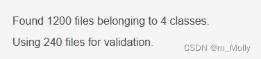
2.加载数据

关键点：（1）函数image_dataset_from_directory的使用；（2）划分训练集和验证集；

batch_size = 32
img_height = 224
img_width = 224
# 按比例分割训练集
train_ds = tf.keras.preprocessing.image_dataset_from_directory(
    data_dir,
    validation_split=0.2,
    subset="training",
    seed=123,
    image_size=(img_height, img_width),
    batch_size=batch_size)

# 按比例分割验证集
val_ds = tf.keras.preprocessing.image_dataset_from_directory(
    data_dir,
    validation_split=0.2,
    subset="validation",
    seed=123,
    image_size=(img_height, img_width),
    batch_size=batch_size)

# 查看指定数据集的标签名称
class_names = train_ds.class_names
print(class_names)

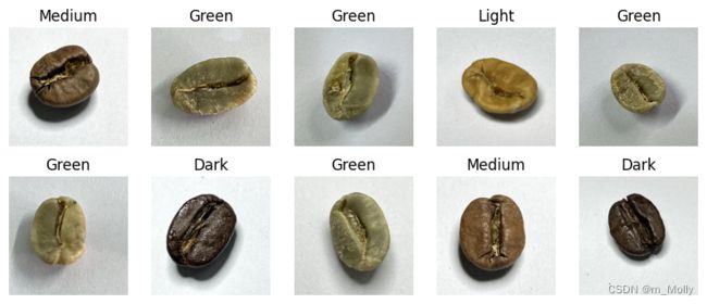
3.可视化数据

随机显示数据集内的图片，以及查看数据的shape值

plt.figure(figsize=(10, 4))  # 图形的宽为10高为5

for images, labels in train_ds.take(1):
    for i in range(10):
        
        ax = plt.subplot(2, 5, i + 1)  

        plt.imshow(images[i].numpy().astype("uint8"))
        plt.title(class_names[labels[i]])
        
        plt.axis("off")

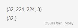
for image_batch, labels_batch in train_ds:
    print(image_batch.shape)
    print(labels_batch.shape)
    break

4.配置数据集

• shuffle() ：打乱数据，关于此函数的详细介绍可以参考：https://zhuanlan.zhihu.com/p/42417456
• prefetch() ：预取数据，加速运行
• cache() ：将数据集缓存到内存当中，加速运行

AUTOTUNE = tf.data.AUTOTUNE

train_ds = train_ds.cache().shuffle(1000).prefetch(buffer_size=AUTOTUNE)
val_ds   = val_ds.cache().prefetch(buffer_size=AUTOTUNE)

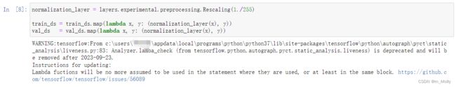
normalization_layer = layers.experimental.preprocessing.Rescaling(1./255)

train_ds = train_ds.map(lambda x, y: (normalization_layer(x), y))
val_ds   = val_ds.map(lambda x, y: (normalization_layer(x), y))

image_batch, labels_batch = next(iter(val_ds))
first_image = image_batch[0]

# 查看归一化后的数据
print(np.min(first_image), np.max(first_image))

我在运行的时候，有关于正则表达式的警告提示，不知道咋回事。

5. 构建VGG-16网络结构

(1)VGG优缺点分析：

● VGG优点

VGG的结构非常简洁，整个网络都使用了同样大小的卷积核尺寸（3x3）和最大池化尺寸（2x2）。

● VGG缺点

1)训练时间过长（我发现了，CPU跑太难了），调参难度大。2)需要的存储容量大，不利于部署。例如存储VGG-16权重值文件的大小为500多MB，不利于安装到嵌入式系统中。

(2)调用方式：官方模型调用，or 自己写代码搭建

(3)网络结构：

# 官方模型调用
# model = tf.keras.applications.VGG16(weights='imagenet')
# model.summary()

# 自己写代码搭建
model = models.Sequential([
    layers.experimental.preprocessing.Rescaling(1./255, input_shape=(img_height, img_width, 3)),
    
    layers.Conv2D(64, (3, 3), activation='relu', padding='same', input_shape=(img_height, img_width, 3)), # 卷积层1，卷积核3*3 
    layers.Conv2D(64, (3, 3), activation='relu', padding='same', input_shape=(img_height, img_width, 3)), # 卷积层2，卷积核3*3  
    layers.MaxPooling2D((2, 2), strides=(2,2)),               # 池化层1，2*2采样
    
    layers.Conv2D(128, (3, 3), activation='relu', padding='same'),  # 卷积层2，卷积核3*3
    layers.Conv2D(128, (3, 3), activation='relu', padding='same'),  # 卷积层2，卷积核3*3
    layers.MaxPooling2D((2, 2), strides=(2,2)),               # 池化层2，2*2采样
    
    layers.Conv2D(256, (3, 3), activation='relu', padding='same'),  # 卷积层2，卷积核3*3
    layers.Conv2D(256, (3, 3), activation='relu', padding='same'),  # 卷积层2，卷积核3*3
    layers.Conv2D(256, (3, 3), activation='relu', padding='same'),  # 卷积层2，卷积核3*3
    layers.MaxPooling2D((2, 2), strides=(2,2)),               # 池化层2，2*2采样
    
    layers.Conv2D(512, (3, 3), activation='relu', padding='same'),  # 卷积层2，卷积核3*3
    layers.Conv2D(512, (3, 3), activation='relu', padding='same'),  # 卷积层2，卷积核3*3
    layers.Conv2D(512, (3, 3), activation='relu', padding='same'),  # 卷积层2，卷积核3*3
    layers.MaxPooling2D((2, 2), strides=(2,2)),               # 池化层2，2*2采样
    
    layers.Conv2D(512, (3, 3), activation='relu', padding='same'),  # 卷积层2，卷积核3*3
    layers.Conv2D(512, (3, 3), activation='relu', padding='same'),  # 卷积层2，卷积核3*3
    layers.Conv2D(512, (3, 3), activation='relu', padding='same'),  # 卷积层2，卷积核3*3
    layers.MaxPooling2D((2, 2), strides=(2,2)),               # 池化层2，2*2采样
    
    layers.Flatten(),
    layers.Dense(4096, activation='relu'),                      
    layers.Dense(4096, activation='relu'),
    layers.Dense(len(class_names),activation='softmax')               # 输出层，输出预期结果
])

model.summary()  # 打印网络结构

6.训练

(1)设置loss函数、优化器、评估指标

● 损失函数（loss）：用于衡量模型在训练期间的准确率。

● 优化器（optimizer）：决定模型如何根据其看到的数据和自身的损失函数进行更新。

● 指标（metrics）：用于监控训练和测试步骤。以下示例使用了准确率，即被正确分类的图像的比率。

# 设置初始学习率
initial_learning_rate = 1e-4

lr_schedule = tf.keras.optimizers.schedules.ExponentialDecay(
        initial_learning_rate, 
        decay_steps=30,      # 敲黑板！！！这里是指 steps，不是指epochs
        decay_rate=0.92,     # lr经过一次衰减就会变成 decay_rate*lr
        staircase=True)

# 设置优化器
opt = tf.keras.optimizers.Adam(learning_rate=initial_learning_rate)

model.compile(optimizer=opt,
              loss=tf.keras.losses.SparseCategoricalCrossentropy(from_logits=True),
              metrics=['accuracy'])

(2)训练模型

VGG-16数据量比较大，本来应该用GPU跑的，但是我没有，所以只能用CPU慢慢的跑，大概跑了不到4个小时。训练结果很差。

epochs = 20

history = model.fit(
    train_ds,
    validation_data=val_ds,
    epochs=epochs
)

7. 可视化结果

acc = history.history['accuracy']
val_acc = history.history['val_accuracy']

loss = history.history['loss']
val_loss = history.history['val_loss']

epochs_range = range(epochs)

plt.figure(figsize=(12, 4))
plt.subplot(1, 2, 1)
plt.plot(epochs_range, acc, label='Training Accuracy')
plt.plot(epochs_range, val_acc, label='Validation Accuracy')
plt.legend(loc='lower right')
plt.title('Training and Validation Accuracy')

plt.subplot(1, 2, 2)
plt.plot(epochs_range, loss, label='Training Loss')
plt.plot(epochs_range, val_loss, label='Validation Loss')
plt.legend(loc='upper right')
plt.title('Training and Validation Loss')
plt.show()

8.其他尝试

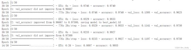
（1）尝试用之前的课程里的训练方法训练，但是CPU速度跑不过来，跑一个epoch的时间将近45分钟了还没跑完，所以后续有时间跑完了，再来更新。

10.26更新：一整晚开着，早上起来以为泡好了，结果训练到epoch=24时候，突然断开了…但能看到accuracy已经增加到0.97了。所以有空的时候再试试。