线性回归、逻辑回归以及感知机的Python实现和比较分析

线性回归

线性回归是回归问题中最基础的一个部分，它通过对一系列特征进行线性关系的操作来拟合一个能够刻画数据集的超平面。如图所示的例子，对于散落在坐标系里的每一个点，它的$x$坐标可以看成是它的特征，而它的$y$坐标则是对应的label值，我们需要对这一组数据进行很好的刻画，才能使得我们在拿到一组新数据时可以准确的预测它的值。在这里，我们采用的是线性回归的方式，即$y=\theta x+b$,因此，二维里就是一条直线。

下面我们将线性回归归纳到一般的情况下，即$h_{\theta }(x)={\theta }_1{x}_1+{\theta }_2{x}_2+......+{\theta }_n{x}_n+b={\theta }^{T}x+b$,其中$\theta =[{\theta }_1,{\theta }_2,......{\theta }_n]$是回归的系数，$b$是偏差值，一般保持不变。对于样本$x^i$,它的特征为$[x_1^i,x_2^i,......,x_n^i]$,对于这样的线性回归方程，采用的代价函数是平均误差平方和，公式如下，
$$J(\theta )=\frac{1}{2m}\sum _{i=0}^m(h_{\theta }(x^i)-y^i{)}^2$$
有了如上的代价函数，下一步需要做的就是最小化此平均误差平方和，在这里采用的是梯度下降，以下是对$\theta$以及$b$的分别求偏导，
$$\frac{\partial J(\theta )}{\partial \theta }=\frac{1}{m}\sum _{i=0}^m{x}^i(h_{\theta }(x^i)-y^i)$$
$$\frac{\partial J(\theta )}{\partial b}=\frac{1}{m}\sum _{i=0}^m(h_{\theta }(x^i)-y^i)$$
由于$\frac{1}{m}$在数据集固定时是一个定值，因此在采用梯度下降算法进行求解最小值的时候将它视为常数，有如下的梯度下降计算方式，
$$\theta =\theta -\alpha \frac{\partial J(\theta )}{\partial \theta }$$
$$b=b-\frac{\partial J(\theta )}{\partial b}$$
这里的$\alpha$为学习率也就是迭代的步长，通过每一步沿着代价函数的负梯度方向进行优化，最终可以得到一个最优的代价函数值，此时的$\theta$以及$b$就作为线性回归模型的回归系数以及偏差值。具体的python实现代码如下，

import numpy as np

class linear_model(object):
    def __init__(self,X,y):
        self.X = np.mat(X)
        self.y = np.mat(y)
        self.number = len(X)
        self.length = len(X[0])
        self.theta = np.ones((self.length,1))
        self.bias = 0.1
        self.train()

    def cost_function(self,X,y):
        result = np.dot(X,self.theta)
        minus_val = y - result
        cost = 0.5*sum(np.array(minus_val)**2)
        if np.isnan(cost):
            return np.inf
        return cost

    def gradientdescent(self,alpha):
        result = np.dot(self.X,self.theta) + self.bias
        #print(result)
        fro_part = result - self.y
        all_gradient = np.dot(self.X.transpose(),fro_part)
        #print(all_gradient)
        self.theta = self.theta - alpha*all_gradient
        self.bias = self.bias - alpha*fro_part


    def train(self,iterations=10000,alpha=0.01,method=0):
        for k in range(iterations):
            if method == 0:
                self.gradientdescent(alpha)

    def predict(self,X_test):
        #print(np.dot(X_test,self.theta))
        return np.dot(X_test,self.theta)

X = [[1.50] ,[2.00],[2.50],[3.00],[3.50],[4.00],[6.00]]
y = [[6.450],[7.450],[8.450],[9.450],[11.450],[15.450],[18.450]]
X_test = [[2.5],[6.0]]
y_test = [[8.450],[18.450]]
y = linear_model(X,y)
y_test1 = y.predict(X_test)
cost = y.cost_function(X_test,y_test)
print(y_test1)
print(cost)

逻辑回归

对于线性回归，我们一般用它来进行回归预测一定的值，不能够作为分类器来使用。但我们通过分析，可以知道线性回归产生的是一个超平面，如果这个超平面可以将不同的两类点分开，那么他就可以作为一个分类器。通过一定的变化，就可以将线性组合的模式应用于分类上，也即是逻辑回归。这里，引入一个sigmoid函数，它是一个0-1之间的S型曲线，在二分类中，可以用此来描述每个特征点属于类别1的概率。如图为sigmoid函数的示意图，

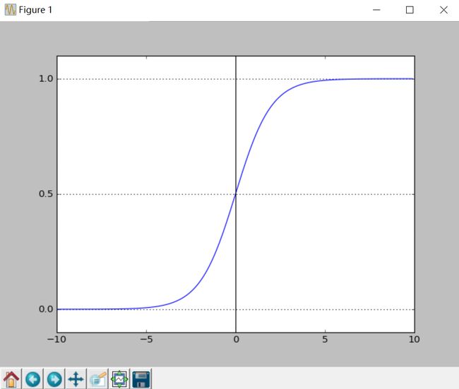
这个sigmoid函数定义为
$$f(x)=\frac{1}{1+e^{-x}}$$
再由线性回归的$h_{\theta }(x)={\theta }_1{x}_1+{\theta }_2{x}_2+......+{\theta }_n{x}_n+b={\theta }^{T}x+b$带入到$f(x)$得到新的$h_{\theta }(x)$为$\frac{1}{1+e^{-(\theta x+b)}}$，这就是它的预测模型，根据$h_{\theta }(x)$可以计算出预测的概率值。
那么如何训练这个模型呢？由于我们把它看作是类别的概率，那么我们可以采用似然估计的方式，似然函数如下，
$$\prod _{i=1}^N[\pi (x_i){]}^{y_i}[1-\pi (x_i){]}^{1-y_i}$$
上述式子中的$\pi (x_i)$表示的是在特征$x_i$下类别为1的概率。接着取对数似然函数$L(\theta )$，有
$$\sum _{i=1}^N[y_{i}log\pi (x_i)+(1-y_i)log(1-\pi (x_i))]$$
那么我们需要最大化似然函数，也就是求$L(\theta )$的极大值，即求$-L(\theta )$的极小值，采用梯度下降的方法即可解决这样的问题。通过计算$J(\theta ,b)$=$-L(\theta )$的偏导数如下，具体推导可参见此链接
$$\frac{\partial J(\theta ,b)}{\partial \theta }=\sum _{i=0}^N{x}^i(h_{\theta }(x^i)-y^i)$$
$$\frac{\partial J(\theta ,b)}{\partial b}=\sum _{i=0}^N(h_{\theta }(x^i)-y^i)$$
同样采用形如线性回归的梯度下降即可优化求得参数$\theta$和b的值。
实现的代码如下，

import numpy as np
import matplotlib.pyplot as plt

class Logistic_reg(object):
    def __init__(self,X,y):
        self.X = X
        self.y = y
        self.b = 0.1
        self.length = len(X[0])
        self.num = len(X)
        self.theta = np.ones((self.length,1))

    def sigmoid(self,re):
        return 1.0 / (1.0 + np.exp(re))

    def cost_function(self):
        cost_sum = 0.0
        for i in range(self.num):
            cost_tem = self.y[i]*np.exp(self.sigmoid(np.dot(self.theta,np.array(self.X[i]))+self.b)) + \
                       (1 - self.y[i]) * np.exp(1 - self.sigmoid(np.dot(self.theta,np.array(self.X[i]))+self.b))
            cost_sum += cost_tem
        return -1 * cost_sum / self.num

    def gradientdescent(self,alpha):
        mat_X = np.mat(self.X)
        mat_y = np.mat(self.y)
        result = self.sigmoid(np.dot(mat_X, self.theta) + self.b)
        # print(result)
        fro_part = result - mat_y
        all_gradient = np.dot(mat_X.transpose(), fro_part)
        # print(all_gradient)
        self.theta = self.theta - alpha * all_gradient
        self.b = self.b - alpha * fro_part

    def stoc_grad_ascent_one(self,alpha): #随机梯度下降
        dataIndex = list(range(self.num))
        for i in range(self.num):
            randIndex = int(np.random.uniform(0, len(dataIndex)))
            h = self.sigmoid(np.dot(self.theta.transpose(),np.array(self.X[i]))+self.b)  # 数值计算
            error =  h - self.y[i]
            split_x = [[j] for j in self.X[i]]
            self.theta = self.theta - alpha * error * np.array(split_x)
            self.b = self.b - alpha * error
            del (dataIndex[randIndex])


    def train(self,iterations=100,alpha=0.1,method=1):
        for k in range(iterations):
            if method == 0:
                self.gradientdescent(alpha)
            if method == 1:
                self.stoc_grad_ascent_one(alpha)
        return self.theta,self.b


    def predict(self,X_test):
        val = self.sigmoid(np.dot(self.theta.transpose(),np.array(X_test)) + self.b)
        return 1 if val > 0.5 else 0


X = [[-0.017612,14.053064],[-1.395634,4.662541],[-0.752157,6.538620],[-1.322371,7.152853],[0.423363,11.054677],
     [0.406704,7.067335],[0.667394,12.741452],[-2.460150,6.866805],[0.569411,9.548755],[-0.026632,10.427743]]

y = [[0],[1],[0],[0],[0],[1],[0],[1],[0],[0]]

lr = Logistic_reg(X,y)
theat,b = lr.train()
print(theat)
print(b)

xcord1 = []
ycord1 = []
xcord2 = []
ycord2 = []
for i in range(len(y)):
    if y[i][0] == 1:
        xcord1.append(X[i][0])
        ycord1.append(X[i][1])
    else:
        xcord2.append(X[i][0])
        ycord2.append(X[i][1])
fig = plt.figure()
ax = fig.add_subplot(111)
ax.scatter(xcord1, ycord1,s=30, c='red', marker='s')
ax.scatter(xcord2, ycord2, s=30, c='green')
x = np.arange(-3, 3, 0.1)
b_mean = np.mean(b)
print(b_mean)
y = (-theat[0, 0] - theat[1, 0] * x) / b_mean #b[0, 0]  #matix
ax.plot(x, y)
plt.xlabel('X1')
plt.ylabel('X2')
plt.show()

感知机

感知机是根据输入实例的特征向量 x 对其进行二类分类的线性模型：
$$h_{\theta }(x)=sign({\theta }_1{x}_1+{\theta }_2{x}_2+......+{\theta }_n{x}_n+b)=sign({\theta }^{T}x+b)$$
$sign(x)$函数标准如下,
$$sign(x)=\{\begin{array}{ll}1,& \text{if x >=0}\\ -1,& \text{if x < 0}\end{array}$$
感知机模型对应于输入空间（特征空间）中的分离超平面 $\theta x+b=0$其中$\theta$是超平面的法向量，b是超平面的截距。
可见感知机是一种线性分类模型，属于判别模型。
感知机学习的重要前提假设是训练数据集是线性可分的。
感知机学的策略是极小化损失函数。
损失函数的一个自然选择是误分类点的总数。但是，这样的损失函数不是参数 $\theta$, b的连续可导的函数，不易于优化。所以通常是选择误分类点到超平面 S 的总距离：
$$L(\theta ,b)=-\sum _{x_i\in M}{y}_i(\theta x_i+b)$$
学习的策略就是求得使 $L(\theta ,b)$ 为最小值的$\theta$和 b。其中 M 是误分类点的集合。
首先，任意选取一个超平面${\theta }_0$,$b_0$,然后用梯度下降法不断地极小化目标函数。极小化的过程中不是一次使 M 中所有误分类点得梯度下降，而是一次随机选取一个误分类点，使其梯度下降。梯度计算如下。
$$\frac{\partial L(\theta ,b)}{\partial \theta }=-\sum _{x_i\in M}{x}_i{y}_i$$
$$\frac{\partial L(\theta ,b)}{\partial b}=-\sum _{x_i\in M}{y}_i$$
随机选取一个误分类点(xi,yi)，对$\theta$,b进行更新：
$$\theta \leftarrow \theta +\eta x_i{y}_i$$
$$b\leftarrow b+\eta y_i$$
其中$\eta$为学习率。
实现的代码如下：

import numpy as np

class Perceptrom(object):
    def __init__(self,X,y):
        self.X = np.array(X)
        self.length = len(X[0])
        self.y = np.array(y)
        self.w = np.ones((self.length))
        self.b = 0

    def process(self,delta,iterations=100):
        for i in range(iterations):
            choice = -1
            for j in range(len(self.X)):
                if np.sign(np.dot(self.w,self.X[j])+self.b) != self.y[j]:
                    choice = j
                    break
            if choice == -1:
                break
            self.w = self.w + delta * self.y[choice] * self.X[choice]
            self.b = self.b + delta * self.y[choice]

    def predict(self,x_test):
        x_test = np.array(x_test)
        return np.sign(np.dot(self.w,x_test)+self.b)


x_train = [[0.5,0],[0,0.5],[1,0.5],[0.5,1]]
y_train = [-1,-1,1,1]
x_test = [1,1]
perceptron = Perceptrom(x_train,y_train)
perceptron.process(1,100)
y = perceptron.predict(x_test)
print(y)

比较分析

总体上来说，三种虽然是属于不同的任务，而且设计的思路也不太相同，但他们的最终求解形式却几乎相似，可能的原因是他们设计的基础都是基于线性的函数$\theta x+b$。
对于PLA即感知机，它是对线性可分的数据集十分有效，但只能用于线性可分的数据集。
对于逻辑回归，相较于PLA，它不要求数据集线性可分，同时它十分容易优化，而且，解释性也比较强，工程上多使用。
对于线性回归，它十分简单，易于优化，解释性较好。

引用

【1】https://blog.csdn.net/wgdzz/article/details/46462813
【2】https://blog.csdn.net/liulina603/article/details/78676723
【3】https://www.cnblogs.com/GuoJiaSheng/p/3928160.html
【4】李航–统计学习方法