乘波前行的问题

1.问题：

考虑两个信号叠加在一起，比如，一个是工频信号50Hz，一个是叠加的高频信号比如有3KHz，简单起见，两个信号都是幅值固定的标准的正弦波，现在我们期望得到那个高频信号，相对工频信号的相对时域波形，它会是什么样的？它的幅值会抖动吗？它会发生类似红移的效应吗？你怎么验算这个操作？

2.尝试构建数学公式

#!/usr/bin/env python3
# -*- coding: utf-8 -*-
# paramsIn => resultOut 
#
import json
import binascii
import numpy as np;
import sys
import struct
import numpy as np
import matplotlib.pyplot as plt
import signal_2048_two_sin

# 绘制信号和包络
def showTwoPairSignals(t, x, spectrum_before, amplitude_envelope, spectrum_after, freqScale, fs):
    freq = np.arange(0, 1024*(10000.0/2048), 10000.0/2048)
    fig, axs = plt.subplots(2, 2, figsize=(10, 8))
    axs[0, 0].plot(t, x)
    axs[0, 0].set_xlabel('Time (s)')
    axs[0, 0].set_ylabel('Amplitude')
    axs[0, 0].set_title('Original Signal')

    axs[1, 0].plot(freq, spectrum_before)
    axs[1, 0].set_xlabel('Frequency (Hz)')
    axs[1, 0].set_ylabel('Amplitude')
    axs[1, 0].set_title('Spectrum Before Transformation')
    axs[1, 0].set_xlim(0, fs/2)

    axs[0, 1].plot(t, amplitude_envelope)
    axs[0, 1].set_xlabel('Time (s)')
    axs[0, 1].set_ylabel('Amplitude')
    axs[0, 1].set_title('Amplitude Envelope')

    axs[1, 1].plot(freq, spectrum_after)
    axs[1, 1].set_xlabel('Frequency (Hz)')
    axs[1, 1].set_ylabel('Amplitude')
    axs[1, 1].set_title('Spectrum After Transformation')
    axs[1, 1].set_xlim(0, fs/2)

    plt.tight_layout()
    plt.show()

def calc_envelope(fft_complex_result, scale_fft, center_fft, zoomOfFreq):
    print(len(fft_complex_result))
    data_array = fft_complex_result;
    center_freq = center_fft/scale_fft;
    zoomOfFreq = zoomOfFreq/scale_fft;


    #频谱进行数字带通滤波
    min_freq = center_freq - zoomOfFreq;
    max_freq = center_freq + zoomOfFreq;
    if(min_freq <0): min_freq = 0;
    if(max_freq>=(len(data_array)//2)): max_freq =len(data_array)//2;
    for i in range(len(data_array)//2): #注意data_array包含对称的频谱。
        if(imax_freq): 
                data_array[i] = 0+0j;
                data_array[-1*i] = 0+0j;
            #no else

    # 幅角变换
    X = data_array;
    phase_shift = np.zeros(len(X))
    for idx in np.arange(0, len(X)//2):
        phase_shift[idx] = -np.angle(X[-idx])
    X_corrected = X * np.exp( 1j * phase_shift)
    
    # 转回时域
    sampleDataFilted  = np.real(np.fft.ifft(X_corrected)); #我不知道为什么不取abs，但是既有的电机时域数据去零点的结果是正确的。
    amplitude_spectrum = [(abs(x)/len(sampleDataFilted)) for x in sampleDataFilted]
    amplitude_spectrum = np.clip(amplitude_spectrum, 0, 65535).astype(np.uint16)

    # 傅里叶变换
    X_of_Envelope = np.fft.fft(amplitude_spectrum)  # 计算原始信号的傅里叶变换
    X_of_Envelope = X_of_Envelope[:len(X_of_Envelope)//2]
    absFFTOfEnvelope = [abs(item)/len(X_of_Envelope) for item in X_of_Envelope];
        
    # to hex again 
    # 将浮点数组转换为 2 字节uint16编码的二进制数据
    ba = amplitude_spectrum.tobytes()
    hex_data = binascii.hexlify(ba).decode('utf-8')
    root = {
        'binData':hex_data,
        'pt':len(hex_data)/2/2, #hex=>byte /2 byte=>uint16 /2
        'byte_len': len(hex_data),
        'scale': (scale_fft*(len(hex_data)/2))
    }

    # out put  json obj: root is ready 
    # it should turn into str => python variable: resultOut
    #######################################################################################

    # json => str
    json_string = json.dumps(root)
    print(json_string);
    resultOut = json_string;
    return (json_string, amplitude_spectrum, absFFTOfEnvelope);

(signal, FFT_result, FFT_abs) = signal_2048_two_sin.genSignal(2048, 2000, 1800)
(envelopeHex, envelope_result, absFFTOfEnvelope) = calc_envelope(FFT_result, 10000/2048., 2000, 250);
print(envelope_result)


showTwoPairSignals(np.arange(0, 2048.0/10000, 1/10000), signal, FFT_abs[:len(FFT_abs)//2], envelope_result, absFFTOfEnvelope, 10000.0/2048, 10000.0)



#其中：signal_2048_two_sin.genSignal(2048, 2000, 1800)的代码参见下文

import math
import wave
import struct
import numpy as np
import matplotlib.pyplot as plt


def genSignal(pt, freq1, freq2):
    # 采样率和采样点数
    sample_rate = 10000
    num_samples = 2048

    # 信号频率和振幅
    frequency_1 = freq1
    frequency_2 = freq2
    amplitude = 0.5

    # 计算每个采样点的时间间隔
    time_interval = 1 / sample_rate

    # 初始化采样点列表
    samples = []
    signal = []
    # 生成采样点
    for i in range(num_samples):
        t = i * time_interval
        value = amplitude * math.sin(2 * math.pi * frequency_1 * t) + amplitude * math.sin(2 * math.pi * frequency_2 * t)
        scaled_value = round(value * 32767)  # 缩放到S16范围
        if(scaled_value>=32767):
            scaled_value = 32767
        if(scaled_value<=-32767):
            scaled_value = 32767
        signal.append(scaled_value)
        samples.append(struct.pack('

2.1实际显示效果：

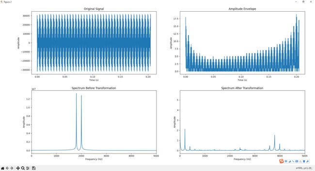
原始波形在左侧，右侧的时域波形似乎完全不对，它应该频率很低才对。但是频谱显示，右侧的峰线确实在左移。我错在哪里了？

上面那个滤波处理，我没有选高通滤波，而是企图直接抹掉频域的一根根谱线，此时的幅角变换我弄错了，对吧？ 

2.1 幅角变换的原则

刚刚了解到一点，如果你直接操作谱线，你需要保证原有的谱线之间的相位关系，保持不变。因为FFT的结果未截断前呈现对称性。所以，你如果改了第0条谱线，你需要把FFT结果中，倒数第一条谱线做同步修改。

2.2 高频信号同步红移的物理意义

现在我们打算做这个操作：

1.我们把高频谱线完全左移到０Hz，然后此时，我们看到的波形，物理意义是什么？

考虑机械振动问题。你对时域采样按某个采样率采样后。这是不是意味着，你达到了更改采样率的目的？同时还滤掉了信号的低频分量？近似于标题的乘波？我们看看那样做的效果。