强化学习-赵世钰(三):贝尔曼最优方程【Bellman Optimal Equation】【贝尔曼最优方程符合收缩映射理论-->可通过迭代法求解最优State Values-->得到最优策略】

强化学习的目的是寻找最优策略。这里学习贝尔曼最优公式需要重点关注两个概念和一个工具:
- 两个概念:optimal state value和optimal policy
- 一个基本工具:the Bellman optimality equation (BOE)
一、Motivating examples
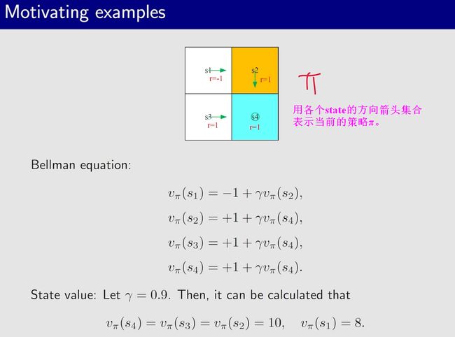
First, we calculate the state values of the given policy. In particular, the Bellman equation of this policy is
υ π ( s 1 ) = − 1 + γ υ π ( s 2 ) , υ π ( s 2 ) = + 1 + γ υ π ( s 4 ) , υ π ( s 3 ) = + 1 + γ υ π ( s 4 ) , υ π ( s 4 ) = + 1 + γ v π ( s 4 ) . \begin{gathered} \upsilon_{\pi}(s_1) =-1+\gamma\upsilon_\pi(s_2), \\ \upsilon_{\pi}(s_{2}) =+1+\gamma\upsilon_\pi(s_4), \\ \upsilon_{\pi}(s_{3}) =+1+\gamma\upsilon_\pi(s_4), \\ \begin{aligned}\upsilon_{\pi}(s_{4})\end{aligned} =+1+\gamma v_\pi(s_4). \end{gathered} υπ(s1)=−1+γυπ(s2),υπ(s2)=+1+γυπ(s4),υπ(s3)=+1+γυπ(s4),υπ(s4)=+1+γvπ(s4).
Let γ = 0.9. It can be easily solved that
v π ( s 4 ) = v π ( s 3 ) = v π ( s 2 ) = 10 , v π ( s 1 ) = 8. \begin{aligned}&v_\pi(s_4)=v_\pi(s_3)=v_\pi(s_2)=10,\\&v_\pi(s_1)=8.\end{aligned} vπ(s4)=vπ(s3)=vπ(s2)=10,vπ(s1)=8.
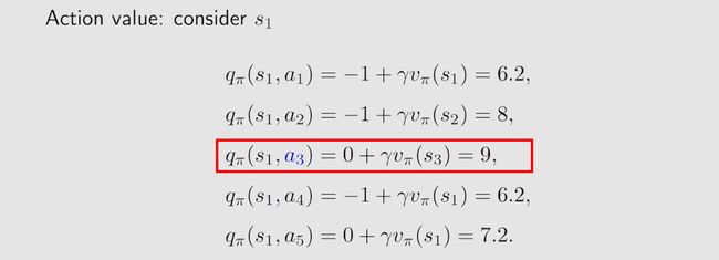
Second, we calculate the action values for state s 1 s_1 s1:
q π ( s 1 , a 1 ) = − 1 + γ v π ( s 1 ) = 6.2 , q π ( s 1 , a 2 ) = − 1 + γ v π ( s 2 ) = 8 , q π ( s 1 , a 3 ) = 0 + γ v π ( s 3 ) = 9 , q π ( s 1 , a 4 ) = − 1 + γ v π ( s 1 ) = 6.2 , q π ( s 1 , a 5 ) = 0 + γ v π ( s 1 ) = 7.2. \begin{gathered} q_\pi(s_1,a_1) =-1+\gamma v_\pi(s_1)=6.2, \\ q_\pi(s_1,a_2) =-1+\gamma v_\pi(s_2)=8, \\ q_\pi(s_1,a_3) =0+\gamma v_\pi(s_3)=9, \\ q_\pi(s_1,a_4) =-1+\gamma v_\pi(s_1)=6.2, \\ q_\pi(s_1,a_5) =0+\gamma v_\pi(s_1)=7.2. \end{gathered} qπ(s1,a1)=−1+γvπ(s1)=6.2,qπ(s1,a2)=−1+γvπ(s2)=8,qπ(s1,a3)=0+γvπ(s3)=9,qπ(s1,a4)=−1+γvπ(s1)=6.2,qπ(s1,a5)=0+γvπ(s1)=7.2.
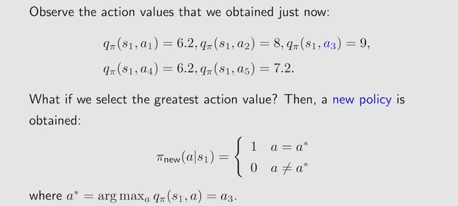
It is notable that action a 3 a_3 a3 has the greatest action value:
q π ( s 1 , a 3 ) ≥ q π ( s 1 , a i ) , for all i ≠ 3. q_\pi(s_1,a_3)\geq q_\pi(s_1,a_i),\quad\text{ for all }i\neq3. qπ(s1,a3)≥qπ(s1,ai), for all i=3.
Therefore, we can update the policy to select a 3 a_3 a3 at s 1 s_1 s1.

每一次迭代的过程中,每一个state都选择action value最大的action,最终就会得到最优的Policy。
二、最优策略/optimal policy
state value可以用来衡量一个policy的好坏,对于策略 π 1 \pi_1 π1 和策略 π 2 \pi_2 π2 来说,倘若在所有的状态 s s s 下,都存在 v π 1 ( s ) ≥ v π 2 ( s ) v_{\pi_1}(s)\geq v_{\pi_2}(s) vπ1(s)≥vπ2(s) 那么可得策略 π 1 \pi_1 π1优于策略 π 2 \pi_2 π2 。因此最优策略 π ∗ \pi^* π∗ 就是,在所有的状态 s s s 下,均优于其他所有的策略 π \pi π。

上述定义表明,相对于所有其他策略,最优策略对于每个状态都具有最大的状态值。这个定义也引发了许多问题:
- 存在性:最优策略是否存在?
- 唯一性:最优策略是否唯一?
- 随机性:最优策略是随机的还是确定性的?
- 算法:如何获得最优策略和最优状态值?
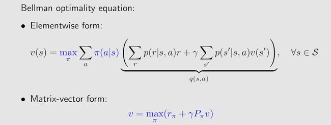
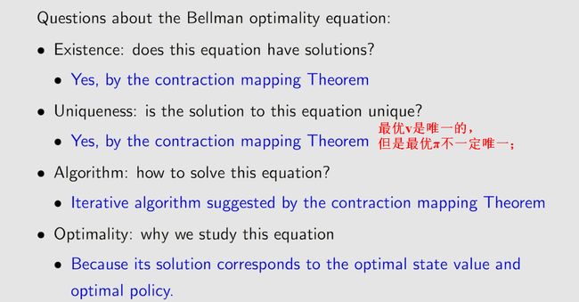
三、贝尔曼最优公式【Bellman Optimality Equation】
1、贝尔曼公式/Bellman Equation
对于贝尔曼公式来说,求解state value时是依赖于一个给定的π;

2、贝尔曼最优公式/Bellman Optimality Equation
对于贝尔曼最优公式来说,π是不定的,是需要求解的参数;
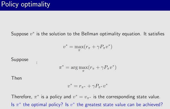
v ( s ) = max π ( s ) ∈ Π ( s ) ∑ a ∈ A π ( a ∣ s ) ( ∑ r ∈ R p ( r ∣ s , a ) r + γ ∑ s ′ ∈ S p ( s ′ ∣ s , a ) v ( s ′ ) ) \begin{aligned}v(s)&=\max_{\pi(s)\in\Pi(s)}\sum_{a\in\mathcal{A}}\pi(a|s)\left(\sum_{r\in\mathcal{R}}p(r|s,a)r+\gamma\sum_{s'\in\mathcal{S}}p(s'|s,a)v(s')\right)\end{aligned} v(s)=π(s)∈Π(s)maxa∈A∑π(a∣s)(r∈R∑p(r∣s,a)r+γs′∈S∑p(s′∣s,a)v(s′)) 公式的含义是:当Policy π π π 取某一个最优化值时,State Value v ( s ) v(s) v(s) 可以取到最大值。


BOE 很棘手但又优雅!
- 为什么优雅?它以一种优雅的方式描述了最优策略和最优状态值。
- 为什么棘手?右侧有一个最大化,可能不容易看出如何计算。
- 有许多问题需要回答:
- 算法:如何解决这个方程?
- 存在性:这个方程是否有解?
- 唯一性:这个方程的解是否唯一?
- 最优性:它与最优策略有什么关系?
3、压缩/收缩映射定理【Contraction mapping theorem】
不动点
压缩/收缩映射
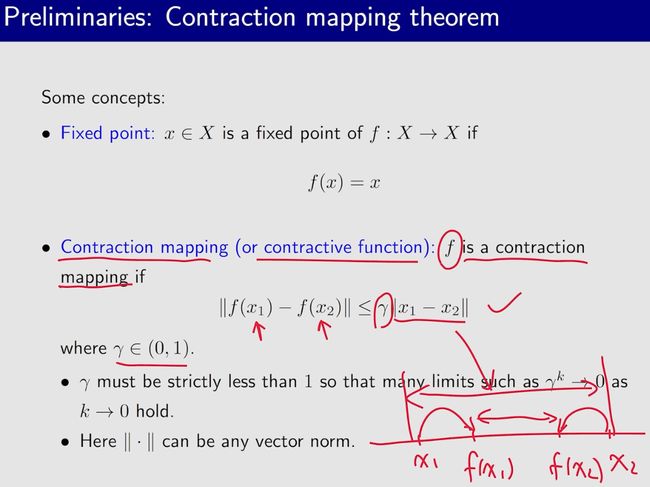
∣ ∣ f ( x 1 ) − f ( x 2 ) ∣ ∣ ≤ γ ∣ ∣ x 1 − x 2 ∣ ∣ ||f(x_1)-f(x_2)||\leq\gamma||x_1-x_2|| ∣∣f(x1)−f(x2)∣∣≤γ∣∣x1−x2∣∣
- 其中 γ ∈ ( 0 , 1 ) \gamma\in(0,1) γ∈(0,1);
- γ \gamma γ必须是严格小于1,这样许多极限 γ k → 0 \gamma^k\to0 γk→0当 k → 0 k\to0 k→0成立;
- 这里 ∣ ∣ ⋅ ∣ ∣ ||\cdot|| ∣∣⋅∣∣可以是任意vector norm;
示例:首先,对于标量来说

其次,对于向量来说
预备知识:Contraction mapping theorem
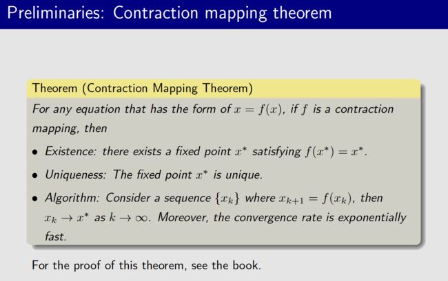
对于任意符合 x = f ( x ) x=f(x) x=f(x) 格式的方程,如果 f f f 是收缩映射,那么:
- 存在性:存在一个不动点 x ∗ x^* x∗ 满足 f ( x ∗ ) = x ∗ f(x^*)=x^* f(x∗)=x∗;
- 唯一性:这个不动点 x ∗ x^* x∗ 是唯一的;
- 算法:迭代式算法 x k + 1 = f ( x k ) x_{k+1}=f(x_k) xk+1=f(xk),最终可以收敛到不动点处;

两个例子
- 对于标量来说: x = 0.5 x x=0.5x x=0.5x, 其中 f ( x ) = 0.5 x f(x)=0.5x f(x)=0.5x 并且 x ∈ R x\in R x∈R, x ∗ = 0 x^*=0 x∗=0是一个唯一 (unique) 的fixed point, 它可以通过迭代式的方式求解
x k + 1 = 0.5 x k x_{k+1}=0.5x_k xk+1=0.5xk
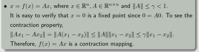
- 对于向量来说, x = A x x=Ax x=Ax,其中 f ( x ) = A x f(x)=Ax f(x)=Ax,且 x ∈ R n x\in R^n x∈Rn, A ∈ R n × n A\in R^{n\times n} A∈Rn×n,并且 ∣ ∣ A ∣ ∣ < 1 ||A||<1 ∣∣A∣∣<1, x ∗ = 0 x^*=0 x∗=0是唯一的不动点,它可以通过迭代式求解
x k + 1 = A x k x_{k+1}=Ax_k xk+1=Axk
4、求解贝尔曼最优公式
4.1 最大化贝尔曼最优公式右侧
首先固定 υ ( s ′ ) \upsilon(s') υ(s′),因为系统模型参数 p ( r ∣ s , a ) p(r|s,a) p(r∣s,a)、 p ( s ′ ∣ s , a ) p(s'|s,a) p(s′∣s,a)都是已知的, r r r(reward)、 γ \gamma γ(discount rate)都是给定的,所以 q ( s , a ) q(s,a) q(s,a) 是常数,为了使得右侧取到最大,则使得右项最大时的 π π π 策略也可以确定下来了。
4.2 解贝尔曼最优公式
从4.1的分析中可知,如果固定 υ ( s ′ ) \upsilon(s') υ(s′),那么贝尔曼最优公式的右侧的最大值就可以确定了。
可见右侧的最大值时取决于 υ ( s ′ ) \upsilon(s') υ(s′),也就是说右侧项是 υ ( s ′ ) \upsilon(s') υ(s′) 的函数。
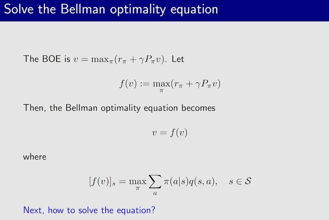
上式中 f ( v ) f(v) f(v) 是一个向量, [ f ( v ) ] s [f(v)]_s [f(v)]s 表示向量中对应的元素state s s s 的值是 max π ∑ a π ( a ∣ s ) q ( s , a ) \begin{aligned}\max_\pi\sum_a\pi(a|s)q(s,a)\end{aligned} πmaxa∑π(a∣s)q(s,a)。
4.3 应用“压缩映射定理”解贝尔曼最优公式
首先要证明贝尔曼最优方程中的 v = f ( v ) v=f(v) v=f(v) 是一个 Contraction Mapping。

∵ ∵ ∵ 通过证明可以得到: ∥ f ( v 1 ) − f ( v 2 ) ∥ ≤ γ ∥ v 1 − v 2 ∥ \|f(v_1)-f(v_2)\|\leq\color{red}{\gamma}\|v_1-v_2\| ∥f(v1)−f(v2)∥≤γ∥v1−v2∥,其中 γ \gamma γ 是 discount rate;
∴ ∴ ∴ v = f ( v ) v=f(v) v=f(v) 是Contraction Mapping。

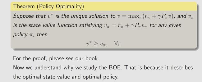
由于贝尔曼最优方程符合Contraction mapping theorem,所以:
- 存在性:存在一个解 v ∗ v^* v∗;
- 唯一性: v ∗ v^* v∗是唯一的;
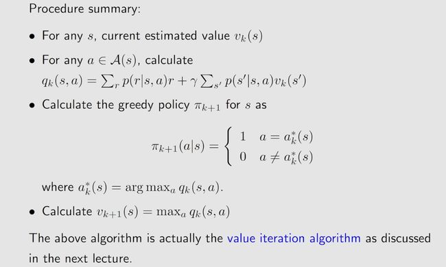
- 算法:State Value 可以通过迭代式算法 v k + 1 = f ( v k ) = max π ( r π + γ P π v k ) \begin{aligned}v_{k+1}=f(v_k)=\max_{\pi}(r_\pi+\gamma P_\pi v_k)\end{aligned} vk+1=f(vk)=πmax(rπ+γPπvk) 最终收敛到唯一解 v ∗ v^* v∗ 处;

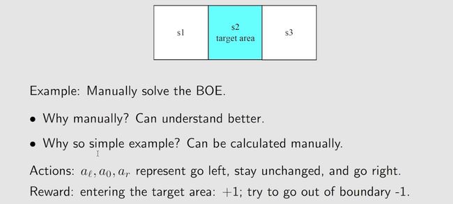
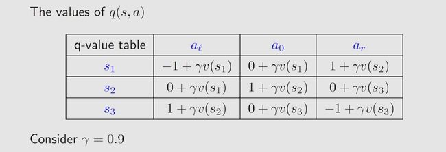
4.4 案例:求解贝尔曼最优公式

四、最优策略/Optimal Policy
贝尔曼最优公式是一个特殊的贝尔曼公式。
贝尔曼最优公式对应的策略是最优策略。

五、最优策略的决定因素

当γ比较大时,会比较远视,得到的return中远期的reward比重会相对大一些;
当γ比较小时,会比较短视,得到的return中近期的reward权重会相对大一些;


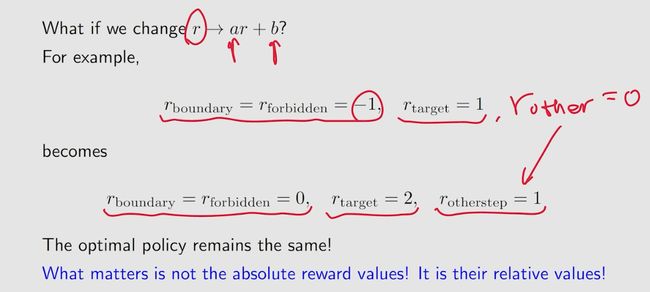

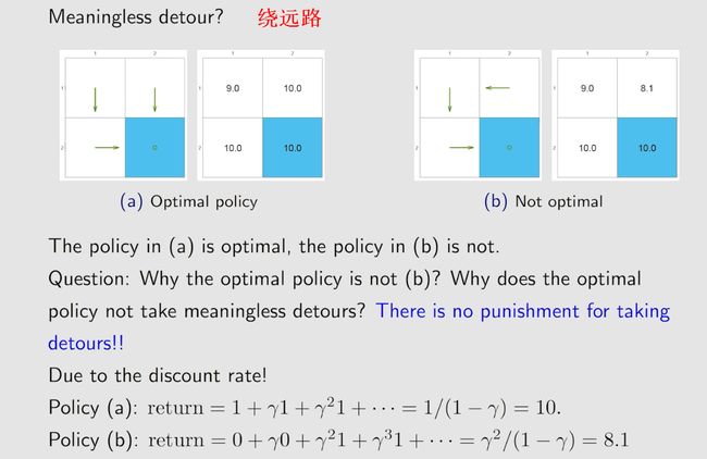
在设计reward的时候,即使将默认r设计为0,也不会绕远路,因为除了r来约束不要绕远路,γ的存在也会限制不会绕远路,因为越绕远路,得到的reward越晚,最后计算得到的return越小。
3.1 Motivating example: How to improve policies?

Consider the policy shown in Figure 3.2. Here, the orange and blue cells represent the forbidden and target areas, respectively. The policy here is n o t not not g o o d good good because it selects a 2 a_{2} a2 ( rightward) at state s 1 s_1 s1. How can we improve the given policy to obtain a better policy? The answer lies in state values and action values.
I n t u i t i o n Intuition Intuition: It is intuitively clear that the policy can improve if it selects a 3 a_3 a3(downward) instead of a 2 a_2 a2(rightward) at s 1 . s_1. s1. This is because moving downward enables the agent to avoid entering the forbidden area.
M a t h e m a t i c s Mathematics Mathematics: The above intuition can be realized based on the calculation of state values and action values.
This example illustrates that we can obtain a better policy if we update the policy to select the action with the g r e a t e s t greatest greatest a c t i o n v a l u e . action~value. action value. This is the basic idea of many reinforcement learning algorithms.
This example is very simple in the sense that the given policy is only not good for state s 1 . s_1. s1. If the policy is also not good for the other states, will selecting the action with the greatest action value still generate a better policy? Moreover, whether there always exist optimal policies? What does an optimal policy look like? We will answer all of these questions in this chapter.
3.2 Optimal state values and optimal policies
While the ultimate goal of reinforcement learning is to obtain optimal policies, it is necessary to first define what an optimal policy is. 【强化学习的最终目标是获得最优策略,但首先需要定义什么是最优策略。】
The defnition is based on state values.
In particular, consider two given policies π 1 \pi_{1} π1 and π 2 \pi_{2} π2. If the state value of π 1 \pi_{1} π1 is greater than or equal to that of π 2 \pi_2 π2 for any state,then π 1 \pi_{1} π1 is said to be better than π 2 \pi_{2} π2. :【考虑给定的两个策略 π 1 \pi_{1} π1和 π 2 \pi_{2} π2, 如果对于任何状态在策略 π 1 \pi_{1} π1下的状态值都大于或等于 π 2 \pi_{2} π2, π 1 \pi_{1} π1被认为比 π 2 \pi_{2} π2更好。】
v π 1 ( s ) ≥ v π 2 ( s ) , for all s ∈ S , \begin{aligned}v_{\pi_1}(s)\geq v_{\pi_2}(s),\quad\text{ for all }s\in\mathcal{S},\end{aligned} vπ1(s)≥vπ2(s), for all s∈S,
Furthermore, if a policy is better than all the other possible policies, then this policy is optimal.【如果一项政策比所有其他可能的政策都要好,那么这项政策就是最优的。】
Definition 3.1 (Optimal policy and optimal state value). A A A p o l i c y π ∗ i s o p t i m a l i f policy\:\pi^*~is~optimal~if policyπ∗ is optimal if v π ∗ ( s ) ≥ v π ( s ) f o r a l l s ∈ S a n d f o r a n y o t h e r p o l i c y π . T h e s t a t e v a l u e s o f π ∗ a r e t h e v_{\pi^*}(s)\geq v_\pi(s)\:for\:all\:s\in\mathcal{S}\:and\:for\:any\:other\:policy\:\pi.\:The\:state\:values\:of\:\pi^*\:are\:the vπ∗(s)≥vπ(s)foralls∈Sandforanyotherpolicyπ.Thestatevaluesofπ∗arethe o p t i m a l optimal optimal s t a t e state state v a l u e s . values. values.
The above definition indicates that an optimal policy has the greatest state value for every state compared to all the other policies. This definition also leads to many questions:
- Existence: Does the optimal policy exist?
- Uniqueness: Is the optimal policy unique?
- Stochasticity: Is the optimal policy stochastic or deterministic?
- Algorithm: How to obtain the optimal policy and the optimal state values?
These fundamental questions must be clearly answered to thoroughly understand optimal policies.
For example, regarding the existence of optimal policies, if optimal policies do not exist, then we do not need to bother to design algorithms to find them.
3.3 Bellman optimality equation【贝尔曼最优方程】
The tool for analyzing optimal policies and optimal state values is the Bellman optimality equation (BOE).
By solving this equation, we can obtain optimal policies and optimal state values. 【通过解决这个方程,我们可以得到最优策略和最优状态值。】
We next present the expression of the BOE and then analyze it in detail.
贝尔曼方程:
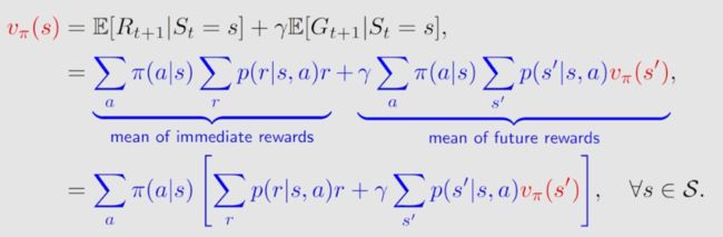
v π ( s ) = E [ R t + 1 ∣ S t = s ] + γ E [ G t + 1 ∣ S t = s ] = ∑ a ∈ A π ( a ∣ s ) ∑ r ∈ R p ( r ∣ s , a ) r ⏟ mean of immediate rewards + γ ∑ a ∈ A π ( a ∣ s ) ∑ s ′ ∈ S p ( s ′ ∣ s , a ) v π ( s ′ ) , ⏟ mean of future rewards = ∑ a ∈ A π ( a ∣ s ) [ ∑ r ∈ R p ( r ∣ s , a ) r + γ ∑ s ′ ∈ S p ( s ′ ∣ s , a ) v π ( s ′ ) ] , for all s ∈ S \begin{aligned} \color{red}{v_{\pi}(s)}&=\mathbb{E}[R_{t+1}|S_t=s]+\gamma\mathbb{E}[G_{t+1}|S_t=s] \\[2ex] &=\underbrace{\sum_{a\in\mathcal{A}}\pi(a|s)\sum_{r\in\mathcal{R}}p(r|s,a)r}_{\text{mean of immediate rewards}}+\underbrace{\gamma\sum_{a\in\mathcal{A}}\pi(a|s)\sum_{s'\in\mathcal{S}}p(s'|s,a)v_{\pi}(s'),}_{\text{mean of future rewards}}\\ &=\sum_{a\in\mathcal{A}}\pi(a|s)\left[\sum_{r\in\mathcal{R}}p(r|s,a)r+\gamma\sum_{s'\in\mathcal{S}}p(s'|s,a)v_{\pi}(s')\right],\quad\text{for all }s\in\mathcal{S} \end{aligned} vπ(s)=E[Rt+1∣St=s]+γE[Gt+1∣St=s]=mean of immediate rewards a∈A∑π(a∣s)r∈R∑p(r∣s,a)r+mean of future rewards γa∈A∑π(a∣s)s′∈S∑p(s′∣s,a)vπ(s′),=a∈A∑π(a∣s)[r∈R∑p(r∣s,a)r+γs′∈S∑p(s′∣s,a)vπ(s′)],for all s∈S
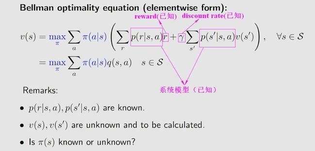
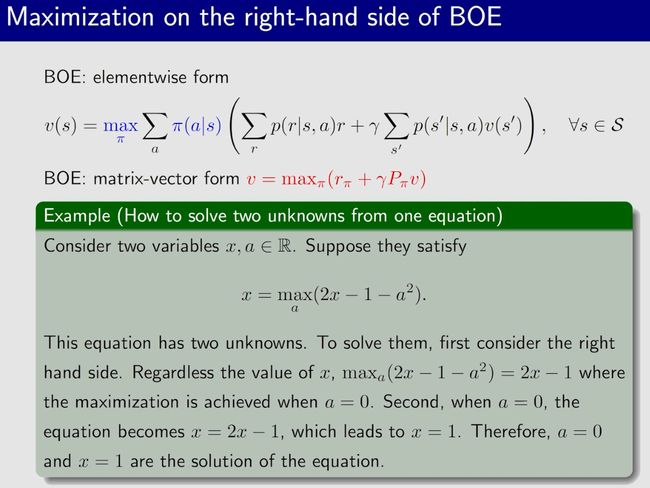
For every s ∈ S s\in\mathcal{S} s∈S, the elementwise expression of the BOE(贝尔曼最优方程) is
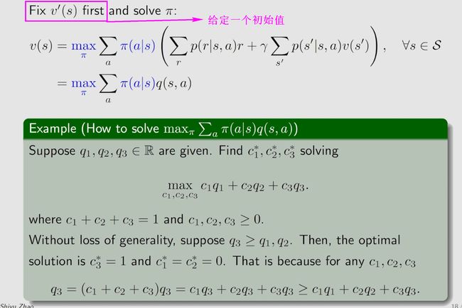
υ ( s ) = max π ( s ) ∈ Π ( s ) ∑ a ∈ A π ( a ∣ s ) ( ∑ r ∈ R p ( r ∣ s , a ) r + γ ∑ s ′ ∈ S p ( s ′ ∣ s , a ) v ( s ′ ) ) = max π ( s ) ∈ Π ( s ) ∑ a ∈ A π ( a ∣ s ) q ( s , a ) , \begin{aligned} \upsilon(s)& \begin{aligned}=\max_{\pi(s)\in\Pi(s)}\sum_{a\in\mathcal{A}}\pi(a|s)\left(\sum_{r\in\mathcal{R}}p(r|s,a)r+\gamma\sum_{s'\in\mathcal{S}}p(s'|s,a)v(s')\right)\end{aligned} \\ &=\max_{\pi(s)\in\Pi(s)}\sum_{a\in\mathcal{A}}\pi(a|s)q(s,a), \end{aligned} υ(s)=π(s)∈Π(s)maxa∈A∑π(a∣s)(r∈R∑p(r∣s,a)r+γs′∈S∑p(s′∣s,a)v(s′))=π(s)∈Π(s)maxa∈A∑π(a∣s)q(s,a),
where v ( s ) , v ( s ′ ) v(s),v(s^{\prime}) v(s),v(s′) are unknown variables to be solved and
q ( s , a ) ≐ ∑ r ∈ R p ( r ∣ s , a ) r + γ ∑ s ′ ∈ S p ( s ′ ∣ s , a ) v ( s ′ ) . q(s,a)\doteq\sum_{r\in\mathcal{R}}p(r|s,a)r+\gamma\sum_{s^{\prime}\in\mathcal{S}}p(s^{\prime}|s,a)v(s^{\prime}). q(s,a)≐r∈R∑p(r∣s,a)r+γs′∈S∑p(s′∣s,a)v(s′).
Here, π ( s ) \pi(s) π(s) denotes a policy for state s s s, and Π ( s ) \Pi(s) Π(s) is the set of all possible policies for s s s.
The BOE(贝尔曼最优方程)is an elegant and powerful tool for analyzing optimal policies.
However, it may be nontrivial to understand this equation. For example, this equation has two unknown variables v ( s ) v(s) v(s) and π ( a ∣ s ) \pi(a|s) π(a∣s).
It may be confusing to beginners how to solve two unknown variables from one equation.
Moreover, the BOE is actually a special Bellman equation.
However, it is nontrivial to see that since its expression is quite different from that of the Bellman equation.
We also need to answer the following fundamental questions about the BOE.
- Existence: Does this equation have a solution?
- Uniqueness: Is the solution unique?
- Algorithm: How to solve this equation?
- Optimality: How is the solution related to optimal policies?
Once we can answer these questions, we will clearly understand optimal state values and optimal policies.
3.3.1 Maximization of the right-hand side of the BOE
We next clarify how to solve the maximization problem on the right-hand side of the BOE.
At first glance, it may be confusing to beginners how to solve t w o two two unknown variables v ( s ) v(s) v(s) and π ( a ∣ s ) \pi(a|s) π(a∣s) from o n e one one equation.
In fact, these two unknown variables can be solved one by one.
This idea is illustrated by the following example.
Example 3.1. C o n s i d e r t w o u n k n o w n v a r i a b l e s x , y ∈ R t h a t s a t i s f y 3.1.Consider\:two\:unknown\:variables\:x,y\in\mathbb{R}\:that\:satisfy 3.1.Considertwounknownvariablesx,y∈Rthatsatisfy
x = max y ∈ R ( 2 x − 1 − y 2 ) . \begin{aligned}x&=\max_{y\in\mathbb{R}}(2x-1-y^2).\end{aligned} x=y∈Rmax(2x−1−y2).
T h e f i r s t s t e p i s t o s o l v e y o n t h e r i g h t − h a n d s i d e o f t h e e q u a t i o n . R e g a r d l e s s o f t h e v a l u e The\:first\:step\:is\:to\:solve\:y\:on\:the\:right-hand\:side\:of\:the\:equation.\:Regardless\:of\:the\:value Thefirststepistosolveyontheright−handsideoftheequation.Regardlessofthevalue o f x , w e a l w a y s h a v e max y ( 2 x − 1 − y 2 ) = 2 x − 1 , w h e r e t h e m a x i m u m i s a c h i e v e d w h e n ofx,\:we\:always\:have\:\max_y(2x-1-y^2)=2x-1,\:where\:the\:maximum\:is\:achieved\:when ofx,wealwayshavemaxy(2x−1−y2)=2x−1,wherethemaximumisachievedwhen y = 0. T h e s e c o n d s t e p i s t o s o l v e x . W h e n y = 0 , t h e e q u a t i o n b e c o m e s x = 2 x − 1 y=0.\quad The\:second\:step\:is\:to\:solve\:x.\quad When\:y=0,\:the\:equation\:becomes\:x=2x-1 y=0.Thesecondstepistosolvex.Wheny=0,theequationbecomesx=2x−1, w h i c h l e a d s t o x = 1. T h e r e f o r e , y = 0 a n d x = 1 a r e t h e s o l u t i o n s o f t h e e q u a t i o n . which\:leads\:to\:x=1.\:Therefore,\:y=0\:and\:x=1\:are\:the\:solutions\:of\:the\:equation. whichleadstox=1.Therefore,y=0andx=1arethesolutionsoftheequation.
We now turn to the maximization problem on the right-hand side of the BOE. The BOE in (3.1) can be written concisely as
v ( s ) = max π ( s ) ∈ Π ( s ) ∑ a ∈ A π ( a ∣ s ) q ( s , a ) , s ∈ S . v(s)=\max_{\pi(s)\in\Pi(s)}\sum_{a\in\mathcal{A}}\pi(a|s)q(s,a),\quad s\in\mathcal{S}. v(s)=π(s)∈Π(s)maxa∈A∑π(a∣s)q(s,a),s∈S.
Inspired by Example 3.1, we can first solve the optimal π \pi π on the right-hand side. How to do that? The following example demonstrates its basic idea.
Example 3.2. G i v e n q 1 , q 2 , q 3 ∈ R , w e w o u l d l i k e t o f i n d t h e o p t i m a l v a l u e s o f c 1 , c 2 , c 3 3.2.\:Given\:q_1,q_2,q_3\in\mathbb{R},\:we\:would\:like\:to\:find\:the\:optimal\:values\:of\:c_1,c_2,c_3 3.2.Givenq1,q2,q3∈R,wewouldliketofindtheoptimalvaluesofc1,c2,c3
t o to to m a x i m i z e maximize maximize
∑ i = 1 3 c i q i = c 1 q 1 + c 2 q 2 + c 3 q 3 , \begin{aligned}\sum_{i=1}^3c_iq_i&=c_1q_1+c_2q_2+c_3q_3,\\\end{aligned} i=1∑3ciqi=c1q1+c2q2+c3q3,
w h e r e c 1 + c 2 + c 3 = 1 a n d c 1 , c 2 , c 3 ≥ 0. \begin{aligned}where\:c_1+c_2+c_3=1\:and\:c_1,c_2,c_3\geq0.\end{aligned} wherec1+c2+c3=1andc1,c2,c3≥0.
W i t h o u t l o s s o f g e n e r a l i t y , s u p p o s e t h a t q 3 ≥ q 1 , q 2 . T h e n , t h e o p t i m a l s o l u t i o n i s Without~loss~of~generality,~suppose~that~q_3~\geq~q_1,q_2.~Then,~the~optimal~solution~is Without loss of generality, suppose that q3 ≥ q1,q2. Then, the optimal solution is c 3 ∗ = 1 a n d c 1 ∗ = c 2 ∗ = 0. T h i s i s b e c a u s e \begin{aligned}c_3^*=1~and~c_1^*=c_2^*=0.~This~is~because\end{aligned} c3∗=1 and c1∗=c2∗=0. This is because
q 3 = ( c 1 + c 2 + c 3 ) q 3 = c 1 q 3 + c 2 q 3 + c 3 q 3 ≥ c 1 q 1 + c 2 q 2 + c 3 q 3 q_3=(c_1+c_2+c_3)q_3=c_1q_3+c_2q_3+c_3q_3\geq c_1q_1+c_2q_2+c_3q_3 q3=(c1+c2+c3)q3=c1q3+c2q3+c3q3≥c1q1+c2q2+c3q3
f o r a n y c 1 , c 2 , c 3 . \begin{aligned}for~any~c_1,c_2,c_3.\end{aligned} for any c1,c2,c3.
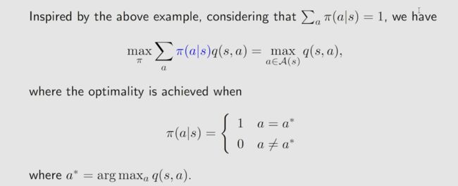
Inspired by the above example, since ∑ a π ( a ∣ s ) = 1 \sum_a\pi(a|s)=1 ∑aπ(a∣s)=1, we have
∑ a ∈ A π ( a ∣ s ) q ( s , a ) ≤ ∑ a ∈ A π ( a ∣ s ) max a ∈ A q ( s , a ) = max a ∈ A q ( s , a ) , \sum_{a\in\mathcal{A}}\pi(a|s)q(s,a)\leq\sum_{a\in\mathcal{A}}\pi(a|s)\max_{a\in\mathcal{A}}q(s,a)=\max_{a\in\mathcal{A}}q(s,a), a∈A∑π(a∣s)q(s,a)≤a∈A∑π(a∣s)a∈Amaxq(s,a)=a∈Amaxq(s,a),
where equality is achieved when
π ( a ∣ s ) = { 1 , a = a ∗ , 0 , a ≠ a ∗ . \left.\pi(a|s)=\left\{\begin{array}{ll}1,&a=a^*,\\0,&a\neq a^*.\end{array}\right.\right. π(a∣s)={1,0,a=a∗,a=a∗.
Here, a ∗ = arg max a q ( s , a ) . a^* = \arg \max _aq( s, a) . a∗=argmaxaq(s,a). In summary, the optimal policy π ( s ) \pi(s) π(s) is the one that selects the action that has the greatest value of q ( s , a ) . q( s, a) . q(s,a).
3.3.2 Matrix-vector form of the BOE
The BOE refers to a set of equations defined for all states. If we combine these equations, we can obtain a concise matrix-vector form, which will be extensively used in this chapter.
The matrix-vector form of the BOE is
υ = max π ∈ Π ( r π + γ P π υ ) , \upsilon=\max_{\pi\in\Pi}(r_\pi+\gamma P_\pi\upsilon), υ=π∈Πmax(rπ+γPπυ),
where v ∈ R ∣ S ∣ v\in\mathbb{R}^{|\mathcal{S}|} v∈R∣S∣ and max is performed in an elementwise manner. The structures of r π r_{\pi} rπ and P π P_{\pi} Pπ are the same as those in the matrix-vector form of the normal Bellman equationı
[ r π ] s ≐ ∑ α ∈ A π ( a ∣ s ) ∑ r ∈ R p ( r ∣ s , a ) r , [ P π ] s , s ′ = p ( s ′ ∣ s ) ≐ ∑ α ∈ A π ( a ∣ s ) p ( s ′ ∣ s , a ) . [r_\pi]_s\doteq\sum_{\alpha\in\mathcal{A}}\pi(a|s)\sum_{r\in\mathcal{R}}p(r|s,a)r,\quad[P_\pi]_{s,s^{\prime}}=p(s'|s)\doteq\sum_{\alpha\in\mathcal{A}}\pi(a|s)p(s'|s,a). [rπ]s≐α∈A∑π(a∣s)r∈R∑p(r∣s,a)r,[Pπ]s,s′=p(s′∣s)≐α∈A∑π(a∣s)p(s′∣s,a).
Since the optimal value of π \pi π is determined by v v v, the right-hand side of (3.2) is a function of $v, $ denoted as
f ( v ) ≐ max π ∈ Π ( r π + γ P π v ) . f(v)\doteq\max_{\pi\in\Pi}(r_\pi+\gamma P_\pi v). f(v)≐π∈Πmax(rπ+γPπv).
Then, the BOE can be expressed in a concise form as
υ = f ( υ ) \upsilon=f(\upsilon) υ=f(υ)
3.3.3 Contraction mapping theorem
Since the BOE can be expressed as a nonlinear equation v = f ( v ) v=f(v) v=f(v), we next introduce the contraction mapping theorem [6] to analyze it. The contraction mapping theorem is a powerful tool for analyzing general nonlinear equations. It is also known as the fixedpoint theorem. Readers who already know this theorem can skip this part. Otherwise the reader is advised to be familiar with this theorem since it is the key to analyzing the BOE.
Consider a function $f( x) , $where x ∈ R d x\in \mathbb{R} ^d x∈Rd and f : R d → R d . f: \mathbb{R} ^d\to \mathbb{R} ^d. f:Rd→Rd.
A point x ∗ x^* x∗ is called a fxed point if
f ( x ∗ ) = x ∗ . f(x^*)=x^*. f(x∗)=x∗.
The interpretation of the above equation is that the map of x ∗ x^* x∗ is itself. This is the reason why x ∗ x^* x∗ is called “fixed”. The function f f f is a c o n t r a c t i o n contraction contraction m a p p i n g mapping mapping (or contractive function) if there exists $\gamma\in ( 0, 1) $ such that
∥ f ( x 1 ) − f ( x 2 ) ∥ ≤ γ ∥ x 1 − x 2 ∥ \|f(x_1)-f(x_2)\|\leq\gamma\|x_1-x_2\| ∥f(x1)−f(x2)∥≤γ∥x1−x2∥
for any x 1 , x 2 ∈ R d . x_1, x_2\in \mathbb{R} ^d. x1,x2∈Rd. In this book, ∥ ⋅ ∥ \|\cdot \| ∥⋅∥denotes a vector or matrix norm.
【强化学习的数学原理】课程:从零开始到透彻理解(完结)
MathFoundationRL/Book-Mathmatical-Foundation-of-Reinforcement-Learning
学习笔记-强化学习4-用Banach不动点定理证明Value-based RL收敛性
【强化学习】强化学习数学基础:贝尔曼最优公式
学习心得-强化学习【贝尔曼最优公式】