Gauss消去法(C++)
文章目录
- 算法描述
-
- 顺序Gauss消去法
- 列选主元Gauss消去法
- 全选主元Gauss消去法
- Gauss-Jordan消去法
- 算法实现
-
- 顺序Gauss消去法
- 列选主元Gauss消去法
- 全选主元Gauss消去法
- 列选主元Gauss-Jordan消去法
- 实例分析
Gauss消去法是求解线性方程组较为有效的方法, 它主要包括两个操作, 即消元和回代. 所谓消元是指将线性方程组转化为与其同解的上三角方程组; 回代是指通过上三角方程组逐个解出方程组的未知数. Gauss消去法通常有顺序Gauss消去法, 列主元Gauss消去法, 全主元Gauss消去法及Gauss-Jordan消去法.
算法描述
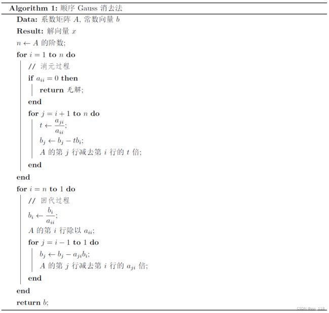
顺序Gauss消去法
顺序Gauss消去法是最简单的Gauss消去法, 其基本步骤如下:
- 将线性方程组的增广矩阵通过行变换, 化简成一个上三角矩阵. 这可以通过交换两行位置或者用一个数乘某一行加到另一行上面来实现.
- 从增广矩阵的最后一行开始, 依次回代, 求出解向量. 回代过程中, 需要将从上方得到的解代入下方方程进行求解.
虽然Gauss消去法可以解决线性方程组的问题, 但是它没有稳定性保证. 如果主元素比较小, 舍入误差可能会累积增大, 从而导致解的误差较大.
算法可描述为伪代码如下:
例 用顺序Gauss消去法求解线性方程组:
{ x + 2 y + 3 z = 1 4 x + 5 y + 6 z = 1 7 x + 8 y = 1 \begin{cases} x+2y+3z=1\\4x+5y+6z=1\\7x+8y=1 \end{cases} ⎩ ⎨ ⎧x+2y+3z=14x+5y+6z=17x+8y=1
利用顺序Gauss消去法得到如下消元过程:
( 1.000000 2.000000 3.000000 1 4.000000 5.000000 6.000000 1 7.000000 8.000000 0.000000 1 ) → ( 1.000000 2.000000 3.000000 1 0.000000 − 3.000000 − 6.000000 − 3 0.000000 − 6.000000 − 21.000000 − 6 ) → ( 1.000000 2.000000 3.000000 1 0.000000 − 3.000000 − 6.000000 − 3 0.000000 0.000000 − 9.000000 0 ) → ( 1.000000 2.000000 0.000000 1 0.000000 − 3.000000 0.000000 − 3 0.000000 0.000000 1.000000 0 ) → ( 1.000000 0.000000 0.000000 − 1 0.000000 1.000000 0.000000 1 0.000000 0.000000 1.000000 0 ) → ( 1.000000 0.000000 0.000000 − 1 0.000000 1.000000 0.000000 1 0.000000 0.000000 1.000000 0 ) \begin{aligned} &\begin{pmatrix} 1.000000&2.000000&3.000000& 1 \\ 4.000000&5.000000&6.000000& 1 \\ 7.000000&8.000000&0.000000& 1 \\ \end{pmatrix}\\\rightarrow& \begin{pmatrix} 1.000000&2.000000&3.000000& 1 \\ 0.000000&-3.000000&-6.000000& -3 \\ 0.000000&-6.000000&-21.000000& -6 \\ \end{pmatrix}\\\rightarrow& \begin{pmatrix} 1.000000&2.000000&3.000000& 1 \\ 0.000000&-3.000000&-6.000000& -3 \\ 0.000000&0.000000&-9.000000& 0 \\ \end{pmatrix}\\\rightarrow& \begin{pmatrix} 1.000000&2.000000&0.000000& 1 \\ 0.000000&-3.000000&0.000000& -3 \\ 0.000000&0.000000&1.000000& 0 \\ \end{pmatrix}\\\rightarrow& \begin{pmatrix} 1.000000&0.000000&0.000000& -1 \\ 0.000000&1.000000&0.000000& 1 \\ 0.000000&0.000000&1.000000& 0 \\ \end{pmatrix}\\\rightarrow& \begin{pmatrix} 1.000000&0.000000&0.000000& -1 \\ 0.000000&1.000000&0.000000& 1 \\ 0.000000&0.000000&1.000000& 0 \\ \end{pmatrix} \end{aligned} →→→→→ 1.0000004.0000007.0000002.0000005.0000008.0000003.0000006.0000000.000000111 1.0000000.0000000.0000002.000000−3.000000−6.0000003.000000−6.000000−21.0000001−3−6 1.0000000.0000000.0000002.000000−3.0000000.0000003.000000−6.000000−9.0000001−30 1.0000000.0000000.0000002.000000−3.0000000.0000000.0000000.0000001.0000001−30 1.0000000.0000000.0000000.0000001.0000000.0000000.0000000.0000001.000000−110 1.0000000.0000000.0000000.0000001.0000000.0000000.0000000.0000001.000000−110
列选主元Gauss消去法
在顺序Gauss消去法中, 并没有选择主元的步骤, 而是按照方程组的顺序进行消元和回代. 这种方法在某些情况下可能会因为计算的顺序而产生数值不稳定性, 导致计算结果与精确解的误差较大. 而且顺序Gauss消去法要求系数矩阵的各阶顺序主子式非零, 而这并不是方程组有解的必要条件. 在列选主元的Gauss消去法中, 每一步计算之前都会增加选择主元的步骤. 这个步骤是为了提高数值稳定性, 避免在计算过程中出现除数为零的情况. 因此, 列选主元的Gauss消去法在计算精度上通常优于顺序高斯消去法. 除此之外, 列选主元Gauss消去法只需要系数矩阵的行列式非零就可以进行计算.
算法可描述为伪代码如下:

例 用列选主元Gauss消去法求解上例线性方程组.
利用列选主元Gauss消去法得到如下消元过程:
( 1.000000 2.000000 3.000000 1 4.000000 5.000000 6.000000 1 7.000000 8.000000 0.000000 1 ) → ( 7.000000 8.000000 0.000000 1 4.000000 5.000000 6.000000 1 1.000000 2.000000 3.000000 1 ) → ( 7.000000 8.000000 0.000000 1 0.000000 0.428571 6.000000 0.428571 0.000000 0.857143 3.000000 0.857143 ) → ( 7.000000 8.000000 0.000000 1 0.000000 0.857143 3.000000 0.857143 0.000000 0.428571 6.000000 0.428571 ) → ( 7.000000 8.000000 0.000000 1 0.000000 0.857143 3.000000 0.857143 0.000000 0.000000 4.500000 0 ) → ( 7.000000 8.000000 0.000000 1 0.000000 0.857143 0.000000 0.857143 0.000000 0.000000 1.000000 0 ) → ( 7.000000 0.000000 0.000000 − 7 0.000000 1.000000 0.000000 1 0.000000 0.000000 1.000000 0 ) → ( 1.000000 0.000000 0.000000 − 1 0.000000 1.000000 0.000000 1 0.000000 0.000000 1.000000 0 ) \begin{aligned} &\begin{pmatrix} 1.000000&2.000000&3.000000& 1 \\ 4.000000&5.000000&6.000000& 1 \\ 7.000000&8.000000&0.000000& 1 \\ \end{pmatrix}\\\rightarrow& \begin{pmatrix} 7.000000&8.000000&0.000000& 1 \\ 4.000000&5.000000&6.000000& 1 \\ 1.000000&2.000000&3.000000& 1 \\ \end{pmatrix}\\\rightarrow& \begin{pmatrix} 7.000000&8.000000&0.000000& 1 \\ 0.000000&0.428571&6.000000& 0.428571 \\ 0.000000&0.857143&3.000000& 0.857143 \\ \end{pmatrix}\\\rightarrow& \begin{pmatrix} 7.000000&8.000000&0.000000& 1 \\ 0.000000&0.857143&3.000000& 0.857143 \\ 0.000000&0.428571&6.000000& 0.428571 \\ \end{pmatrix}\\\rightarrow& \begin{pmatrix} 7.000000&8.000000&0.000000& 1 \\ 0.000000&0.857143&3.000000& 0.857143 \\ 0.000000&0.000000&4.500000& 0 \\ \end{pmatrix}\\\rightarrow& \begin{pmatrix} 7.000000&8.000000&0.000000& 1 \\ 0.000000&0.857143&0.000000& 0.857143 \\ 0.000000&0.000000&1.000000& 0 \\ \end{pmatrix}\\\rightarrow& \begin{pmatrix} 7.000000&0.000000&0.000000& -7 \\ 0.000000&1.000000&0.000000& 1 \\ 0.000000&0.000000&1.000000& 0 \\ \end{pmatrix}\\\rightarrow& \begin{pmatrix} 1.000000&0.000000&0.000000& -1 \\ 0.000000&1.000000&0.000000& 1 \\ 0.000000&0.000000&1.000000& 0 \\ \end{pmatrix} \end{aligned} →→→→→→→ 1.0000004.0000007.0000002.0000005.0000008.0000003.0000006.0000000.000000111 7.0000004.0000001.0000008.0000005.0000002.0000000.0000006.0000003.000000111 7.0000000.0000000.0000008.0000000.4285710.8571430.0000006.0000003.00000010.4285710.857143 7.0000000.0000000.0000008.0000000.8571430.4285710.0000003.0000006.00000010.8571430.428571 7.0000000.0000000.0000008.0000000.8571430.0000000.0000003.0000004.50000010.8571430 7.0000000.0000000.0000008.0000000.8571430.0000000.0000000.0000001.00000010.8571430 7.0000000.0000000.0000000.0000001.0000000.0000000.0000000.0000001.000000−710 1.0000000.0000000.0000000.0000001.0000000.0000000.0000000.0000001.000000−110
全选主元Gauss消去法
全选主元Gauss消去法是在列选主元Gauss消去法的基础上, 进一步扩大主元的搜索区间到整个矩阵, 精度更高, 但需要更多的计算量. 全选主元法选取了矩阵中最大值的元素作为主元, 并进行列变换. 这使得在回代过程中, 未知数的位置可能发生改变, 因此需要同时对未知量的顺序进行变换, 从而增加了计算量. 实际使用时, 完全主元素消去法比列主元素消去法运算量大得多, 全选主元的计算时间大约是列选主元的两倍.
算法可描述为伪代码如下:

例 用全选主元Gauss消去法求解上例线性方程组.
利用全选主元Gauss消去法得到如下消元过程:
( 1.000000 2.000000 3.000000 1 4.000000 5.000000 6.000000 1 7.000000 8.000000 0.000000 1 ) → ( 8.000000 7.000000 0.000000 1 5.000000 4.000000 6.000000 1 2.000000 1.000000 3.000000 1 ) → ( 8.000000 7.000000 0.000000 1 0.000000 − 0.375000 6.000000 0.375 0.000000 − 0.750000 3.000000 0.75 ) → ( 8.000000 0.000000 7.000000 1 0.000000 6.000000 − 0.375000 0.375 0.000000 3.000000 − 0.750000 0.75 ) → ( 8.000000 0.000000 7.000000 1 0.000000 6.000000 − 0.375000 0.375 0.000000 0.000000 − 0.562500 0.5625 ) → ( 8.000000 0.000000 0.000000 8 0.000000 6.000000 0.000000 0 0.000000 0.000000 1.000000 − 1 ) → ( 8.000000 0.000000 0.000000 8 0.000000 1.000000 0.000000 0 0.000000 0.000000 1.000000 − 1 ) → ( 1.000000 0.000000 0.000000 1 0.000000 1.000000 0.000000 0 0.000000 0.000000 1.000000 − 1 ) \begin{aligned} &\begin{pmatrix} 1.000000&2.000000&3.000000& 1 \\ 4.000000&5.000000&6.000000& 1 \\ 7.000000&8.000000&0.000000& 1 \\ \end{pmatrix}\\\rightarrow& \begin{pmatrix} 8.000000&7.000000&0.000000& 1 \\ 5.000000&4.000000&6.000000& 1 \\ 2.000000&1.000000&3.000000& 1 \\ \end{pmatrix}\\\rightarrow& \begin{pmatrix} 8.000000&7.000000&0.000000& 1 \\ 0.000000&-0.375000&6.000000& 0.375 \\ 0.000000&-0.750000&3.000000& 0.75 \\ \end{pmatrix}\\\rightarrow& \begin{pmatrix} 8.000000&0.000000&7.000000& 1 \\ 0.000000&6.000000&-0.375000& 0.375 \\ 0.000000&3.000000&-0.750000& 0.75 \\ \end{pmatrix}\\\rightarrow& \begin{pmatrix} 8.000000&0.000000&7.000000& 1 \\ 0.000000&6.000000&-0.375000& 0.375 \\ 0.000000&0.000000&-0.562500& 0.5625 \\ \end{pmatrix}\\\rightarrow& \begin{pmatrix} 8.000000&0.000000&0.000000& 8 \\ 0.000000&6.000000&0.000000& 0 \\ 0.000000&0.000000&1.000000& -1 \\ \end{pmatrix}\\\rightarrow& \begin{pmatrix} 8.000000&0.000000&0.000000& 8 \\ 0.000000&1.000000&0.000000& 0 \\ 0.000000&0.000000&1.000000& -1 \\ \end{pmatrix}\\\rightarrow& \begin{pmatrix} 1.000000&0.000000&0.000000& 1 \\ 0.000000&1.000000&0.000000& 0 \\ 0.000000&0.000000&1.000000& -1 \\ \end{pmatrix} \end{aligned} →→→→→→→ 1.0000004.0000007.0000002.0000005.0000008.0000003.0000006.0000000.000000111 8.0000005.0000002.0000007.0000004.0000001.0000000.0000006.0000003.000000111 8.0000000.0000000.0000007.000000−0.375000−0.7500000.0000006.0000003.00000010.3750.75 8.0000000.0000000.0000000.0000006.0000003.0000007.000000−0.375000−0.75000010.3750.75 8.0000000.0000000.0000000.0000006.0000000.0000007.000000−0.375000−0.56250010.3750.5625 8.0000000.0000000.0000000.0000006.0000000.0000000.0000000.0000001.00000080−1 8.0000000.0000000.0000000.0000001.0000000.0000000.0000000.0000001.00000080−1 1.0000000.0000000.0000000.0000001.0000000.0000000.0000000.0000001.00000010−1
Gauss-Jordan消去法
Gauss-Jordan消去法是高斯消元法的另一个版本, 其方法与高斯消元法相同. 唯一相异之处是该算法产生出来的矩阵是一个简化行梯阵式, 而不是高斯消元法中的行梯阵式. 相比起高斯消元法, Gauss-Jordan消去法的效率较低, 但可以把方程组的解用矩阵一次过表示出来.
Gauss-Jordan消去法也有顺序, 列选主元和全选主元3种消去方式. 由于列主元素消去法的舍入误差一般已较小, 所以在实际计算中多用列主元素消去法. 故算法实现一般采用列选主元Gauss-Jordan消去法.
算法可描述为伪代码如下:

例 用列选主元Gauss消去法求解上例线性方程组.
利用列选主元Gauss-Jordan消去法得到如下消元过程:
( 1.000000 2.000000 3.000000 1 4.000000 5.000000 6.000000 1 7.000000 8.000000 0.000000 1 ) → ( 7.000000 8.000000 0.000000 1 4.000000 5.000000 6.000000 1 1.000000 2.000000 3.000000 1 ) → ( 1.000000 1.142857 0.000000 0.142857 0.000000 0.428571 6.000000 0.428571 0.000000 0.857143 3.000000 0.857143 ) → ( 1.000000 1.142857 0.000000 0.142857 0.000000 0.857143 3.000000 0.857143 0.000000 0.428571 6.000000 0.428571 ) → ( 1.000000 0.000000 − 4.000000 − 1 0.000000 1.000000 3.500000 1 0.000000 0.000000 4.500000 0 ) → ( 1.000000 0.000000 0.000000 − 1 0.000000 1.000000 0.000000 1 0.000000 0.000000 1.000000 0 ) \begin{aligned} &\begin{pmatrix} 1.000000&2.000000&3.000000& 1 \\ 4.000000&5.000000&6.000000& 1 \\ 7.000000&8.000000&0.000000& 1 \\ \end{pmatrix}\\\rightarrow& \begin{pmatrix} 7.000000&8.000000&0.000000& 1 \\ 4.000000&5.000000&6.000000& 1 \\ 1.000000&2.000000&3.000000& 1 \\ \end{pmatrix}\\\rightarrow& \begin{pmatrix} 1.000000&1.142857&0.000000& 0.142857 \\ 0.000000&0.428571&6.000000& 0.428571 \\ 0.000000&0.857143&3.000000& 0.857143 \\ \end{pmatrix}\\\rightarrow& \begin{pmatrix} 1.000000&1.142857&0.000000& 0.142857 \\ 0.000000&0.857143&3.000000& 0.857143 \\ 0.000000&0.428571&6.000000& 0.428571 \\ \end{pmatrix}\\\rightarrow& \begin{pmatrix} 1.000000&0.000000&-4.000000& -1 \\ 0.000000&1.000000&3.500000& 1 \\ 0.000000&0.000000&4.500000& 0 \\ \end{pmatrix}\\\rightarrow& \begin{pmatrix} 1.000000&0.000000&0.000000& -1 \\ 0.000000&1.000000&0.000000& 1 \\ 0.000000&0.000000&1.000000& 0 \\ \end{pmatrix} \end{aligned} →→→→→ 1.0000004.0000007.0000002.0000005.0000008.0000003.0000006.0000000.000000111 7.0000004.0000001.0000008.0000005.0000002.0000000.0000006.0000003.000000111 1.0000000.0000000.0000001.1428570.4285710.8571430.0000006.0000003.0000000.1428570.4285710.857143 1.0000000.0000000.0000001.1428570.8571430.4285710.0000003.0000006.0000000.1428570.8571430.428571 1.0000000.0000000.0000000.0000001.0000000.000000−4.0000003.5000004.500000−110 1.0000000.0000000.0000000.0000001.0000000.0000000.0000000.0000001.000000−110
算法实现
首先进行预处理如下:
#include 顺序Gauss消去法
/*
 * 顺序Gauss消去法
 * A : 系数矩阵
 * b : 常数向量
 * uA: 系数矩阵消元过程
 * ub: 常数向量消元过程
 * e : 判零标准
 *
 * 返回(bool):
 *  true : 求解失败
 *  false: 求解成功
 *
 * 不检查矩阵维数是否匹配问题
 */
bool Sequential_Gauss(mat A, vec b, vector<mat> &uA, vector<vec> &ub, const double &e = 1e-6)
{
    uA.clear();
    ub.clear();
    uA.push_back(A);
    ub.push_back(b);
    unsigned n(A.n_cols - 1), m(-1);
    // 消元
    for (unsigned i(0); i != n; ++i) // arma::mat的迭代器不太好用, 最后还是用了下标形式, 效率相比迭代器低一些
    {
        if (A.at(i, i) < e && A.at(i, i) > -e)
            return true;
        for (unsigned j(i + 1); j != A.n_cols; ++j)
        {
            double t(A.at(j, i) / A.at(i, i));
            A.at(j, i) = 0;
            b.at(j) -= t * b.at(i);
            for (unsigned k(i + 2); k < A.n_cols; ++k)
                A.at(j, k) -= t * A.at(i, k);
        }
        uA.push_back(A);
        ub.push_back(b);
    }
    // 回代
    do
    {
        if (A.at(n, n) < e && A.at(n, n) > -e)
            return true;
        b.at(n) /= A.at(n, n);
        A.at(n, n) = 1;
        for (unsigned i(0); i != n; ++i)
        {
            b.at(i) -= A.at(i, n) * b.at(n);
            A.at(i, n) = 0;
        }
        uA.push_back(A);
        ub.push_back(b);
    } while (--n != m);
    return false;
}
列选主元Gauss消去法
/*
 * 列选主元Gauss消去法
 * A : 系数矩阵
 * b : 常数向量
 * uA: 系数矩阵消元过程
 * ub: 常数向量消元过程
 * e : 判零标准
 *
 * 返回(bool):
 *  true : 求解失败
 *  false: 求解成功
 *
 * 不检查矩阵维数是否匹配问题
 */
bool Col_Gauss(mat A, vec b, vector<mat> &uA, vector<vec> &ub, const double &e = 1e-6)
{
    uA.clear();
    ub.clear();
    uA.push_back(A);
    ub.push_back(b);
    unsigned n(A.n_cols - 1), m(-1);
    for (unsigned i(0); i != n; ++i) // 消元
    {
        unsigned max(i); // 选列主元
        for (unsigned j(i + 1); j != A.n_cols; ++j)
            if (abs(A.at(j, i)) > abs(A.at(max, i)))
                max = j;
        if (abs(A.at(max, i)) < e)
            return true;
        if (max != i)
        {
            for (unsigned j(i); j != A.n_cols; ++j)
            {
                double t(A.at(i, j));
                A.at(i, j) = A.at(max, j);
                A.at(max, j) = t;
            }
            double t(b.at(max));
            b.at(max) = b.at(i);
            b.at(i) = t;
            uA.push_back(A);
            ub.push_back(b);
        }
        for (unsigned j(i + 1); j != A.n_cols; ++j)
        {
            double t(A.at(j, i) / A.at(i, i));
            A.at(j, i) = 0;
            b.at(j) -= t * b.at(i);
            for (unsigned k(i + 1); k < A.n_cols; ++k)
                A.at(j, k) -= t * A.at(i, k);
        }
        uA.push_back(A);
        ub.push_back(b);
    }
    do // 回代
    {
        if (A.at(n, n) < e && A.at(n, n) > -e)
            return true;
        b.at(n) /= A.at(n, n);
        A.at(n, n) = 1;
        for (unsigned i(0); i != n; ++i)
        {
            b.at(i) -= A.at(i, n) * b.at(n);
            A.at(i, n) = 0;
        }
        uA.push_back(A);
        ub.push_back(b);
    } while (--n != m);
    return false;
}
全选主元Gauss消去法
/*
 * 全选主元Gauss消去法
 * A : 系数矩阵
 * b : 常数向量
 * uA: 系数矩阵消元过程
 * ub: 常数向量消元过程
 * r : 解向量
 * e : 判零标准
 *
 * 返回(bool):
 *  true : 求解失败
 *  false: 求解成功
 *
 * 不检查矩阵维数是否匹配问题
 */
bool All_Gauss(mat A, vec b, vector<mat> &uA, vector<vec> &ub, vec &r, const double &e = 1e-6)
{
    uA.clear();
    ub.clear();
    uA.push_back(A);
    ub.push_back(b);
    r.zeros(A.n_cols);
    unsigned n(A.n_cols - 1), m(-1), *a(new unsigned[A.n_cols]);
    for (unsigned t(0); t < A.n_rows; ++t) // 初始化排序向量
        a[t] = t;
    for (unsigned i(0); i != n; ++i) // 消元
    {
        unsigned x(i), y(i); // 选主元
        for (unsigned j(i); j != A.n_cols; ++j)
            for (unsigned k(i); k != A.n_cols; ++k)
                if (abs(A.at(j, k)) > abs(A.at(x, y)))
                {
                    x = j;
                    y = k;
                }
        if (abs(A.at(x, y)) < e)
        {
            delete[] a;
            return true;
        }
        bool flag(false);
        if (x != i)
        {
            for (unsigned j(i); j < A.n_cols; ++j)
            {
                double t(A.at(x, j));
                A.at(x, j) = A.at(i, j);
                A.at(i, j) = t;
            }
            double t(b.at(x));
            b.at(x) = b.at(i);
            b.at(i) = t;
            flag = true;
        }
        if (y != i)
        {
            for (unsigned j(0); j < A.n_cols; ++j)
            {
                double t(A.at(j, i));
                A.at(j, i) = A.at(j, y);
                A.at(j, y) = t;
            }
            flag = true;
            unsigned t(a[i]);
            a[i] = a[y];
            a[y] = t;
        }
        if (flag)
        {
            uA.push_back(A);
            ub.push_back(b);
        }
        for (unsigned j(i + 1); j != A.n_cols; ++j)
        {
            double t(A.at(j, i) / A.at(i, i));
            A.at(j, i) = 0;
            b.at(j) -= t * b.at(i);
            for (unsigned k(i + 2); k < A.n_cols; ++k)
                A.at(j, k) -= t * A.at(i, k);
        }
        uA.push_back(A);
        ub.push_back(b);
    }
    do // 回代
    {
        if (abs(A.at(n, n)) < e)
        {
            delete[] a;
            return true;
        }
        r.at(a[n]) = b.at(n) /= A.at(n, n);
        A.at(n, n) = 1;
        for (unsigned i(0); i != n; ++i)
        {
            b.at(i) -= A.at(i, n) * b.at(n);
            A.at(i, n) = 0;
        }
        uA.push_back(A);
        ub.push_back(b);
    } while (--n != m);
    delete[] a;
    return false;
}
列选主元Gauss-Jordan消去法
/*
 * 列选主元Gauss-Jordan消去法
 * A : 系数矩阵
 * b : 常数向量
 * uA: 系数矩阵消元过程
 * ub: 常数向量消元过程
 * e : 判零标准
 *
 * 返回(bool):
 *  true : 求解失败
 *  false: 求解成功
 *
 * 不检查矩阵维数是否匹配问题
 */
bool Gauss_Jordan(mat A, vec b, vector<mat> &uA, vector<vec> &ub, const double &e = 1e-6)
{
    uA.clear();
    ub.clear();
    uA.push_back(A);
    ub.push_back(b);
    unsigned n(A.n_cols - 1);
    for (unsigned i(0); i != n; ++i)
    {
        unsigned max(i); // 选列主元
        for (unsigned j(i + 1); j != A.n_cols; ++j)
            if (abs(A.at(j, i)) > abs(A.at(max, i)))
                max = j;
        if (abs(A.at(max, i)) < e)
            return true;
        if (max != i)
        {
            for (unsigned j(i); j != A.n_cols; ++j)
            {
                double t(A.at(i, j));
                A.at(i, j) = A.at(max, j);
                A.at(max, j) = t;
            }
            double t(b.at(max));
            b.at(max) = b.at(i);
            b.at(i) = t;
            uA.push_back(A);
            ub.push_back(b);
        }
        b.at(i) /= A.at(i, i);
        for (unsigned k(i + 1); k != A.n_cols; ++k)
            A.at(i, k) /= A.at(i, i);
        for (unsigned j(i + 1); j < A.n_rows; ++j)
        {
            b.at(j) -= b.at(i) * A.at(j, i);
            for (unsigned k(i + 1); k < A.n_cols; ++k)
                A.at(j, k) -= A.at(i, k) * A.at(j, i);
            A.at(j, i) = 0;
        }
        for (unsigned j(0); j != i; ++j)
        {
            b.at(j) -= b.at(i) * A.at(j, i);
            for (unsigned k(i + 1); k < A.n_cols; ++k)
                A.at(j, k) -= A.at(i, k) * A.at(j, i);
            A.at(j, i) = 0;
        }
        A.at(i, i) = 1;
        uA.push_back(A);
        ub.push_back(b);
    }
    return false;
}
实例分析
用列主元高斯消去法求解方程组
{ 0.101 x 1 + 2.304 x 2 + 3.555 x 3 = 1.183 − 1.347 x 1 + 3.712 x 2 + 4.623 x 3 = 2.137 − 2.835 x 1 + 1.072 x 2 + 5.643 x 3 = 3.035 \begin{cases} 0.101x_1+2.304x_2+3.555x_3=1.183\\ -1.347x_1+3.712x_2+4.623x_3=2.137\\ -2.835x_1+1.072x_2+5.643x_3=3.035 \end{cases} ⎩ ⎨ ⎧0.101x1+2.304x2+3.555x3=1.183−1.347x1+3.712x2+4.623x3=2.137−2.835x1+1.072x2+5.643x3=3.035
代入程序, 求得列主元高斯消元过程如下:
( 0.101000 2.304000 3.555000 1.183 − 1.347000 3.712000 4.623000 2.137 − 2.835000 1.072000 5.643000 3.035 ) → ( − 2.835000 1.072000 5.643000 3.035 − 1.347000 3.712000 4.623000 2.137 0.101000 2.304000 3.555000 1.183 ) → ( − 2.835000 1.072000 5.643000 3.035 0.000000 3.202658 1.941829 0.694974 0.000000 2.342191 3.756038 1.29113 ) → ( − 2.835000 1.072000 5.643000 3.035 0.000000 3.202658 1.941829 0.694974 0.000000 0.000000 2.335926 0.782872 ) → ( − 2.835000 1.072000 0.000000 1.14378 0.000000 3.202658 0.000000 0.0441809 0.000000 0.000000 1.000000 0.335144 ) → ( − 2.835000 0.000000 0.000000 1.12899 0.000000 1.000000 0.000000 0.0137951 0.000000 0.000000 1.000000 0.335144 ) → ( 1.000000 0.000000 0.000000 − 0.398234 0.000000 1.000000 0.000000 0.0137951 0.000000 0.000000 1.000000 0.335144 ) \begin{aligned} \begin{pmatrix} 0.101000&2.304000&3.555000& 1.183 \\ -1.347000&3.712000&4.623000& 2.137 \\ -2.835000&1.072000&5.643000& 3.035 \\ \end{pmatrix}\\\rightarrow \begin{pmatrix} -2.835000&1.072000&5.643000& 3.035 \\ -1.347000&3.712000&4.623000& 2.137 \\ 0.101000&2.304000&3.555000& 1.183 \\ \end{pmatrix}\\\rightarrow \begin{pmatrix} -2.835000&1.072000&5.643000& 3.035 \\ 0.000000&3.202658&1.941829& 0.694974 \\ 0.000000&2.342191&3.756038& 1.29113 \\ \end{pmatrix}\\\rightarrow \begin{pmatrix} -2.835000&1.072000&5.643000& 3.035 \\ 0.000000&3.202658&1.941829& 0.694974 \\ 0.000000&0.000000&2.335926& 0.782872 \\ \end{pmatrix}\\\rightarrow \begin{pmatrix} -2.835000&1.072000&0.000000& 1.14378 \\ 0.000000&3.202658&0.000000& 0.0441809 \\ 0.000000&0.000000&1.000000& 0.335144 \\ \end{pmatrix}\\\rightarrow \begin{pmatrix} -2.835000&0.000000&0.000000& 1.12899 \\ 0.000000&1.000000&0.000000& 0.0137951 \\ 0.000000&0.000000&1.000000& 0.335144 \\ \end{pmatrix}\\\rightarrow \begin{pmatrix} 1.000000&0.000000&0.000000& -0.398234 \\ 0.000000&1.000000&0.000000& 0.0137951 \\ 0.000000&0.000000&1.000000& 0.335144 \\ \end{pmatrix} \end{aligned} 0.101000−1.347000−2.8350002.3040003.7120001.0720003.5550004.6230005.6430001.1832.1373.035 → −2.835000−1.3470000.1010001.0720003.7120002.3040005.6430004.6230003.5550003.0352.1371.183 → −2.8350000.0000000.0000001.0720003.2026582.3421915.6430001.9418293.7560383.0350.6949741.29113 → −2.8350000.0000000.0000001.0720003.2026580.0000005.6430001.9418292.3359263.0350.6949740.782872 → −2.8350000.0000000.0000001.0720003.2026580.0000000.0000000.0000001.0000001.143780.04418090.335144 → −2.8350000.0000000.0000000.0000001.0000000.0000000.0000000.0000001.0000001.128990.01379510.335144 → 1.0000000.0000000.0000000.0000001.0000000.0000000.0000000.0000001.000000−0.3982340.01379510.335144