《机器学习》学习笔记
$4.4中有一个比较容易混淆的问题:
即4.4.2和4.4.3,出现以下概念:
1. Perceptron Training Rule
2. Delta Rule
其中最后的形式都是根据预测误差对输入网络的权重进行一个类似负反馈的调整,因而给人造成错觉,似乎两者是同一的。但是,文中清楚说明了他们的区别,即能否适用于线性不可分(Linearly Separable)网络。
个人理解:首先,前者是对多个样本逐个进行计算(即基于iteration)。从直观上讲,它的确需要样本具有很强的甚至严格的线性可分性,并且学习系数(learning rate)也足够小,才能较为理想地地收敛到目标值;而后者在对全部样本集合D上进行,对其而言假设空间(Hypothesis Space)已经确定,只要有唯一的极小值点,总能通过梯度下降法(Gradient Descent)收敛到这个点,而不管是否样本线性可分(当然线性可分保证了假设空间具有唯一极小值点)。
其次,Perceptron Training Rule和Incremental Gradient Rule除了在忽略阈函数的意义上是一致的。且可以证明IGR方法在针对带sgn阈函数的情形有效,因为它既然能在不含阈函数的情形下将权值收敛到目标点(1或-1附近),对输入进行目标点上的权值确定的线性变换再输入阈函数也能产生合理的值(sgn(1) = 1, sgn(-1) = -1)。
Suppose e[k] = w.*x[k] - y[k], where, k is the index of the sample instance. Theoretically, if the sample set is linear separable, the planes in the hypothesis space should intersect at a definite point on the e = 0 plane, which indicates the solution set of the weights. For E = sigma(k, e[k]^2), it is the sum of these individual simple parabolic surfaces for the samples (a more complex parablic surface). According to the property of parabolic surface, it has unique minimum point, the process to acquire which is inherently the LMS(Least Mean Square) Rule.
One can view learning or approximation of the weights specified by PTR or IGR as a process of applying each paraboloid in the set to corresponding step of gradient descent procedure to move the probing point a bit, if there are enough number of samples and they are highly depictable by linear system, the point is expected to converge to the destination.
Anyway, the BP network training method is very effective, as is pointed out by the book.
In the following part we will see some examples on BP training:
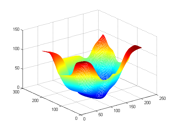
I created a [2, 8, 8, 1] network (with two inputs and one output) to simulate the function z = x*x + y*y
The network allows bias, with transfer functions of its first two layers being sigmoid and of final layer being identical (f(x) = x),
I set momentum coefficient alpha to 0.1, learning rate* 0.2,
After training for 10000 iterations, the graph of the resultant function looks like:

== Network Attributes ==
seed = 1226250528
nIter = 10000
dynRange = 10.000000
alpha = 0.100000
lnorm = 0.200000
nLayers = 4
nNodes[1] = 8
nNodes[2] = 8
------------------------
: Creating network...ok
: Training...ok
: Simulating...ok
The image makes sense. But it's not the end. There are a lot of interesting points in establishing the network, the theoretical explanation for many of them is left unknown. We will look into some of them in the next chapter.