随机抽样一致性算法（RANSAC）资料合集

 本文翻译自维基百科,译者：http://www.cnblogs.com/xrwang/archive/2011/03/09/ransac-1.html,本人在此基础上进行了一些添加和修改。

英文原文地址是：http://en.wikipedia.org/wiki/ransac，如果您英语不错，建议您直接查看原文。
    RANSAC是“RANdom SAmple Consensus（随机抽样一致）”的缩写。它可以从一组包含“局外点”的观测数据集中，通过迭代方式估计数学模型的参数。它是一种不确定的算法——它有一定的概率得出一个合理的结果；为了提高概率必须提高迭代次数。该算法最早由Fischler和Bolles于1981年提出。
    RANSAC的基本假设是：
（1）数据由“局内点”组成，例如：数据的分布可以用一些模型参数来解释；
（2）“局外点”是不能适应该模型的数据；
（3）除此之外的数据属于噪声。
    局外点产生的原因有：噪声的极值；错误的测量方法；对数据的错误假设。
    RANSAC也做了以下假设：给定一组（通常很小的）局内点，存在一个可以估计模型参数的过程；而该模型能够解释或者适用于局内点。

一、示例
    一个简单的例子是从一组观测数据中找出合适的2维直线。假设观测数据中包含局内点和局外点，其中局内点近似的被直线所通过，而局外点远离于直线。简单的最小二乘法不能找到适应于局内点的直线，原因是最小二乘法尽量去适应包括局外点在内的所有点。相反，RANSAC能得出一个仅仅用局内点计算出模型，并且概率还足够高。但是，RANSAC并不能保证结果一定正确，为了保证算法有足够高的合理概率，我们必须小心的选择算法的参数。

左图：包含很多局外点的数据集       右图：RANSAC找到的直线（局外点并不影响结果）

二、概述
    RANSAC算法的输入是一组观测数据，一个可以解释或者适应于观测数据的参数化模型，一些可信的参数。
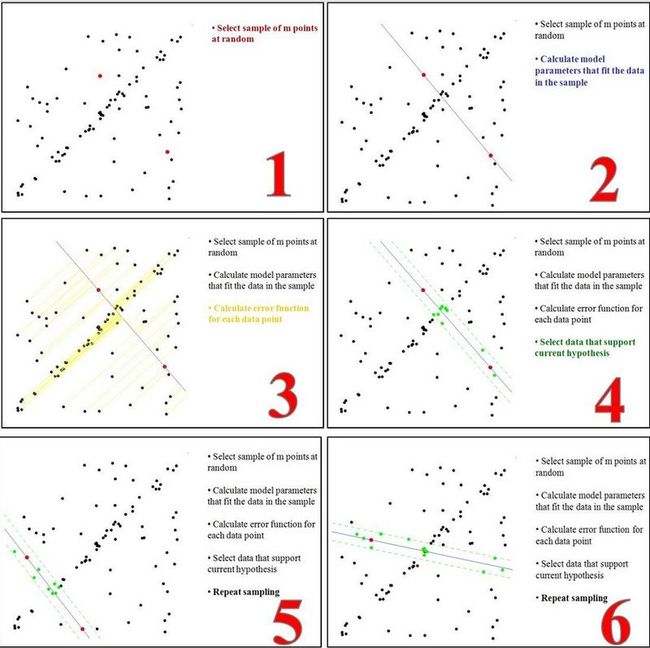
    RANSAC通过反复选择数据中的一组随机子集来达成目标。被选取的子集被假设为局内点，并用下述方法进行验证：
    1.有一个模型适应于假设的局内点，即所有的未知参数都能从假设的局内点计算得出。
    2.用1中得到的模型去测试所有的其它数据，如果某个点适用于估计的模型，认为它也是局内点。
    3.如果有足够多的点被归类为假设的局内点，那么估计的模型就足够合理。
    4.然后，用所有假设的局内点去重新估计模型，因为它仅仅被初始的假设局内点估计过。
    5.最后，通过估计局内点与模型的错误率来评估模型。
    这个过程被重复执行固定的次数，每次产生的模型要么因为局内点太少而被舍弃，要么因为比现有的模型更好而被选用。

整个过程可参考下图： 

三、算法
    伪码形式的算法如下所示：
输入：
data —— 一组观测数据
model —— 适应于数据的模型
n —— 适用于模型的最少数据个数
k —— 算法的迭代次数
t —— 用于决定数据是否适应于模型的阀值
d —— 判定模型是否适用于数据集的数据数目
输出：
best_model —— 跟数据最匹配的模型参数（如果没有找到好的模型，返回null）
best_consensus_set —— 估计出模型的数据点
best_error —— 跟数据相关的估计出的模型错误

iterations = 0
best_model = null
best_consensus_set = null
best_error = 无穷大
while ( iterations < k )
    maybe_inliers = 从数据集中随机选择n个点
    maybe_model = 适合于maybe_inliers的模型参数
    consensus_set = maybe_inliers

    for ( 每个数据集中不属于maybe_inliers的点 ）
        if ( 如果点适合于maybe_model，且错误小于t ）
            将点添加到consensus_set
    if （ consensus_set中的元素数目大于d ）
        已经找到了好的模型，现在测试该模型到底有多好
        better_model = 适合于consensus_set中所有点的模型参数
        this_error = better_model究竟如何适合这些点的度量
        if ( this_error < best_error )
            我们发现了比以前好的模型，保存该模型直到更好的模型出现
            best_model =  better_model
            best_consensus_set = consensus_set
            best_error =  this_error
    增加迭代次数
返回 best_model, best_consensus_set, best_error

    RANSAC算法的可能变化包括以下几种：
    （1）如果发现了一种足够好的模型（该模型有足够小的错误率），则跳出主循环。这样可能会节约计算额外参数的时间。
    （2）直接从maybe_model计算this_error，而不从consensus_set重新估计模型。这样可能会节约比较两种模型错误的时间，但可能会对噪声更敏感。

四、参数
    我们不得不根据特定的问题和数据集通过实验来确定参数t和d。然而参数k（迭代次数）可以从理论结果推断。当我们从估计模型参数时，用p表示一些迭代过程中从数据集内随机选取出的点均为局内点的概率；此时，结果模型很可能有用，因此p也表征了算法产生有用结果的概率。用w表示每次从数据集中选取一个局内点的概率，如下式所示：
    w = 局内点的数目 / 数据集的数目
    通常情况下，我们事先并不知道w的值，但是可以给出一些鲁棒的值。假设估计模型需要选定n个点，wⁿ是所有n个点均为局内点的概率；1 − wⁿ是n个点中至少有一个点为局外点的概率，此时表明我们从数据集中估计出了一个不好的模型。 (1 − wⁿ)^k表示算法永远都不会选择到n个点均为局内点的概率，它和1-p相同。因此，
    1 − p = (1 − wⁿ)^k
    我们对上式的两边取对数，得出
       

值得注意的是，这个结果假设n个点都是独立选择的；也就是说，某个点被选定之后，它可能会被后续的迭代过程重复选定到。这种方法通常都不合理，由此推导出的k值被看作是选取不重复点的上限。例如，要从上图中的数据集寻找适合的直线，RANSAC算法通常在每次迭代时选取2个点，计算通过这两点的直线maybe_model，要求这两点必须唯一。
    为了得到更可信的参数，标准偏差或它的乘积可以被加到k上。k的标准偏差定义为：
   

五、优点与缺点
    RANSAC的优点是它能鲁棒的估计模型参数。例如，它能从包含大量局外点的数据集中估计出高精度的参数。RANSAC的缺点是它计算参数的迭代次数没有上限；如果设置迭代次数的上限，得到的结果可能不是最优的结果，甚至可能得到错误的结果。RANSAC只有一定的概率得到可信的模型，概率与迭代次数成正比。RANSAC的另一个缺点是它要求设置跟问题相关的阀值。
    RANSAC只能从特定的数据集中估计出一个模型，如果存在两个（或多个）模型，RANSAC不能找到别的模型。

六、应用
    RANSAC算法经常用于计算机视觉，例如同时求解相关问题与估计立体摄像机的基础矩阵。

七、参考文献

• Martin A. Fischler and Robert C. Bolles (June 1981). "Random Sample Consensus: A Paradigm for Model Fitting with Applications to Image Analysis and Automated Cartography". Comm. of the ACM 24: 381–395. doi:10.1145/358669.358692. 

• David A. Forsyth and Jean Ponce (2003). Computer Vision, a modern approach. Prentice Hall. ISBN 0-13-085198-1. 

• Richard Hartley and Andrew Zisserman (2003). Multiple View Geometry in Computer Vision (2nd ed.). Cambridge University Press. 

• P.H.S. Torr and D.W. Murray (1997). "The Development and Comparison of Robust Methods for Estimating the Fundamental Matrix". International Journal of Computer Vision 24: 271–300. doi:10.1023/A:1007927408552. 

• Ondrej Chum (2005). "Two-View Geometry Estimation by Random Sample and Consensus". PhD Thesis. http://cmp.felk.cvut.cz/~chum/Teze/Chum-PhD.pdf 

• Sunglok Choi, Taemin Kim, and Wonpil Yu (2009). "Performance Evaluation of RANSAC Family". In Proceedings of the British Machine Vision Conference (BMVC). http://www.bmva.org/bmvc/2009/Papers/Paper355/Paper355.pdf.

八、外部链接

• RANSAC Toolbox for MATLAB. A research (and didactic) oriented toolbox to explore the RANSAC algorithm in MATLAB. It is highly configurable and contains the routines to solve a few relevant estimation problems.

• Implementation in C++ as a generic template.

• RANSAC for Dummies A simple tutorial with many examples that uses the RANSAC Toolbox for MATLAB.

• 25 Years of RANSAC Workshop

九、算法实现（C#、C++）

C# 实现：http://www.cnblogs.com/xrwang/p/SampleOfRansac.html,这篇文章很清晰的介绍了算法的设计步骤，并提供了非常规范的源代码，即便是用C#实现，稍微有点基础的人也能很容将其移植到Ｃ++平台上。强烈推荐。

C++ 实现：网上收集

#include <math.h>
#include "LineParamEstimator.h"

LineParamEstimator::LineParamEstimator(double delta) : m_deltaSquared(delta*delta) {}
/*****************************************************************************/
/*
 * Compute the line parameters  [n_x,n_y,a_x,a_y]
 * 通过输入的两点来确定所在直线，采用法线向量的方式来表示，以兼容平行或垂直的情况
 * 其中n_x,n_y为归一化后，与原点构成的法线向量，a_x,a_y为直线上任意一点
 */
void LineParamEstimator::estimate(std::vector<Point2D *> &data, 
																	std::vector<double> &parameters)
{
	parameters.clear();
	if(data.size()<2)
		return;
	double nx = data[1]->y - data[0]->y;
	double ny = data[0]->x - data[1]->x;// 原始直线的斜率为K，则法线的斜率为-1/k
	double norm = sqrt(nx*nx + ny*ny);
	
	parameters.push_back(nx/norm);
	parameters.push_back(ny/norm);
	parameters.push_back(data[0]->x);
	parameters.push_back(data[0]->y);		
}
/*****************************************************************************/
/*
 * Compute the line parameters  [n_x,n_y,a_x,a_y]
 * 使用最小二乘法，从输入点中拟合出确定直线模型的所需参量
 */
void LineParamEstimator::leastSquaresEstimate(std::vector<Point2D *> &data, 
																							std::vector<double> &parameters)
{
	double meanX, meanY, nx, ny, norm;
	double covMat11, covMat12, covMat21, covMat22; // The entries of the symmetric covarinace matrix
	int i, dataSize = data.size();

	parameters.clear();
	if(data.size()<2)
		return;

	meanX = meanY = 0.0;
	covMat11 = covMat12 = covMat21 = covMat22 = 0;
	for(i=0; i<dataSize; i++) {
		meanX +=data[i]->x;
		meanY +=data[i]->y;

		covMat11	+=data[i]->x * data[i]->x;
		covMat12	+=data[i]->x * data[i]->y;
		covMat22	+=data[i]->y * data[i]->y;
	}

	meanX/=dataSize;
	meanY/=dataSize;

	covMat11 -= dataSize*meanX*meanX;
        covMat12 -= dataSize*meanX*meanY;
	covMat22 -= dataSize*meanY*meanY;
	covMat21 = covMat12;

	if(covMat11<1e-12) {
		nx = 1.0;
	        ny = 0.0;
	}
	else {	    //lamda1 is the largest eigen-value of the covariance matrix 
	           //and is used to compute the eigne-vector corresponding to the smallest
	           //eigenvalue, which isn't computed explicitly.
		double lamda1 = (covMat11 + covMat22 + sqrt((covMat11-covMat22)*(covMat11-covMat22) + 4*covMat12*covMat12)) / 2.0;
		nx = -covMat12;
		ny = lamda1 - covMat22;
		norm = sqrt(nx*nx + ny*ny);
		nx/=norm;
		ny/=norm;
	}
	parameters.push_back(nx);
	parameters.push_back(ny);
	parameters.push_back(meanX);
	parameters.push_back(meanY);
}
/*****************************************************************************/
/*
 * Given the line parameters  [n_x,n_y,a_x,a_y] check if
 * [n_x, n_y] dot [data.x-a_x, data.y-a_y] < m_delta
 * 通过与已知法线的点乘结果，确定待测点与已知直线的匹配程度；结果越小则越符合，为
 * 零则表明点在直线上
 */
bool LineParamEstimator::agree(std::vector<double> &parameters, Point2D &data)
{
	double signedDistance = parameters[0]*(data.x-parameters[2]) + parameters[1]*(data.y-parameters[3]); 
	return ((signedDistance*signedDistance) < m_deltaSquared);
}

RANSAC寻找匹配的代码如下：

/*****************************************************************************/
template<class T, class S>
double Ransac<T,S>::compute(std::vector<S> &parameters, 
													  ParameterEsitmator<T,S> *paramEstimator , 
												    std::vector<T> &data, 
												    int numForEstimate)
{
	std::vector<T *> leastSquaresEstimateData;
	int numDataObjects = data.size();
	int numVotesForBest = -1;
	int *arr = new int[numForEstimate];// numForEstimate表示拟合模型所需要的最少点数，对本例的直线来说，该值为2
	short *curVotes = new short[numDataObjects];  //one if data[i] agrees with the current model, otherwise zero
	short *bestVotes = new short[numDataObjects];  //one if data[i] agrees with the best model, otherwise zero
	

		      //there are less data objects than the minimum required for an exact fit
	if(numDataObjects < numForEstimate) 
		return 0;
        // 计算所有可能的直线，寻找其中误差最小的解。对于100点的直线拟合来说，大约需要100*99*0.5=4950次运算，复杂度无疑是庞大的。一般采用随机选取子集的方式。
	computeAllChoices(paramEstimator,data,numForEstimate,
										bestVotes, curVotes, numVotesForBest, 0, data.size(), numForEstimate, 0, arr);

	   //compute the least squares estimate using the largest sub set
	for(int j=0; j<numDataObjects; j++) {
		if(bestVotes[j])
			leastSquaresEstimateData.push_back(&(data[j]));
	}
        // 对局内点再次用最小二乘法拟合出模型
	paramEstimator->leastSquaresEstimate(leastSquaresEstimateData,parameters);

	delete [] arr;
	delete [] bestVotes;
	delete [] curVotes;	

	return (double)leastSquaresEstimateData.size()/(double)numDataObjects;
}

前面提供的代码实现都是二维情况下形状的拟合。最近我们项目中要使用到三维情况下的直线拟合。可以仿照第一个C#代码编写，但是三维情况下很多判断标准、计算公式都会变化，这一点要注意。我是用的代码是从PCL(point cloud library )中提取出来的，实现思路是一样的，但其中用到了Eigen库中的数据结构来进行计算，基础差的人会比较难读懂，如果有时间我会改成C++ 中的基本数据结构来实现，其实看懂了是很容易改造的。

代码地址：http://www.oschina.net/code/snippet_588162_50399

来自为知笔记(Wiz)