OpenSCAD对象的位移、旋转、拉伸、镜像与颜色设置
Transformation affect the child nodes and as the name implies transforms them in various ways such as moving/rotating or scaling the child. Cascading transformations are used to apply a variety of transforms to a final child. Cascading is achieved by nesting statements i.e.
rotate([45,45,45])
  translate([10,20,30])
    cube(10);
Transformations can be applied to a group of child nodes by using '{' & '}' to enclose the subtree e.g.
 translate([0,0,-5])    or the more compact      translate([0,0,-5]) {
 {                                                 cube(10);
   cube(10);                                       cylinder(r=5,h=10);
   cylinder(r=5,h=10);                           }
 }
Advanced concept
As OpenSCAD uses different libraries to implement capabilities this can introduce some inconsistencies to the F5 preview behaviour of transformations. Traditional transforms (translate, rotate, scale, mirror & multimatrix) are performed using OpenGL in preview, while other more advanced transforms, such as resize, perform a CGAL operation, behaving like a CSG operation affecting the underlying object, not just transforming it. In particular this can affect the display of modifier characters, specifically "#" and "%", where the highlight may not display intuitively, such as highlighting the pre-resized object, but highlighting the post-scaled object.
scale
Scales its child elements using the specified vector. The argument name is optional.
Usage Example:
scale(v = [x, y, z]) { ... }
cube(10);
translate([15,0,0]) scale([0.5,1,2]) cube(10);
resize
resize() is available since OpenSCAD 2013.06. It modifies the size of the child object to match the given x,y, and z.
There is a bug with shrinking in the 2013.06 release, that will be fixed in the next release.
Usage Example:
// resize the sphere to extend 30 in x, 60 in y, and 10 in the z directions.
resize(newsize=[30,60,10]) sphere(r=10);
If x,y, or z is 0 then that dimension is left as-is.
// resize the 1x1x1 cube to 2x2x1
resize([2,2,0]) cube();
If the 'auto' parameter is set to true, it will auto-scale any 0-dimensions to match. For example.
// resize the 1x2x0.5 cube to 7x14x3.5
resize([7,0,0], auto=true) cube([1,2,0.5]);
The 'auto' parameter can also be used if you only wish to auto-scale a single dimension, and leave the other as-is.
// resize to 10x8x1. Note that the z dimension is left alone.
resize([10,0,0], auto=[true,true,false]) cube([5,4,1]);
rotate
Rotates its child 'a' degrees about the origin of the coordinate system or around an arbitrary axis. The argument names are optional if the arguments are given in the same order as specified.
Usage:
rotate(a = deg_a, v = [x, y, z]) { ... }
// or
rotate(deg_a, [x, y, z]) { ... }
rotate(a = [deg_x, deg_y, deg_z]) { ... }
rotate([deg_x, deg_y, deg_z]) { ... }
The 'a' argument (deg_a) can be an array, as expressed in the later usage above; when deg_a is an array, the 'v' argument is ignored. Where 'a' specifies multiple axes then the rotation is applied in the following order: x, y, z.
The optional argument 'v' is a vector and allows you to set an arbitrary axis about which the object will be rotated.
For example, to flip an object upside-down, you can rotate your object 180 degrees around the 'y' axis.
rotate(a=[0,180,0]) { ... }
This is frequently simplified to
rotate([0,180,0]) { ... }
When specifying a single axis the 'v' argument allows you to specify which axis is the basis for rotation. For example, the equivalent to the above, to rotate just around y
rotate(a=180, v=[0,1,0]) { ... }
When specifying mutiple axis, 'v'is a vector defining an arbitrary axis for rotation; this is different from the multiple axis above. For example, rotate your object 45 degrees around the axis defined by the vector [1,1,0],
rotate(a=45, v=[1,1,0]) { ... }
Rotate with a single scalar argument rotates around the Z axis. This is useful in 2D contexts where that is the only axis for rotation. For example:
rotate(45) square(10);
If this is all a bit confusing, this might, or might not, help.
Right-hand grip rule
For the case of:
rotate([a, b, c]) { ... };
"a" is a rotation about the X axis, from the +Z axis, toward the -Y axis. NOTE: NEGATIVE Y.
"b" is a rotation about the Y axis, from the +Z axis, toward the +X axis.
"c" is a rotation about the Z axis, from the +X axis, toward the +Y axis.
These are all cases of the Right Hand Rule. Point your right thumb along the positive axis, your fingers show the direction of rotation.
Thus if "a" is fixed to zero, and "b" and "c" are manipulated appropriately, this is the spherical coordinate system.
So, to construct a cylinder from the origin to some other point (x,y,z):
%cube(10);
x= 10; y = 10; z = 10; // point coordinates of end of cyliner
//
length = sqrt( pow(x, 2) + pow(y, 2) + pow(z, 2) );
b = acos(z/length);
c = (x==0) ? sign(y)*90 : ( (x>0) ? atan(y/x) : atan(y/x)+180 );
//
rotate([0, b, c])
    cylinder(h=length, r=0.5);
translate
Translates (moves) its child elements along the specified vector. The argument name is optional.
IExample
translate(v = [x, y, z]) { ... }
cube(2,center = true);
translate([5,0,0])
  sphere(1,center = true);
mirror
Mirrors the child element on a plane through the origin. The argument to mirror() is the normal vector of a plane intersecting the origin through which to mirror the object.
Function signature:
mirror( [x, y, z] ) { ... }
Examples
rotate([0,0,10]) cube([3,2,1]);
mirror([1,0,0]) translate([1,0,0]) rotate([0,0,10]) cube([3,2,1]);
multmatrix
Multiplies the geometry of all child elements with the given 4x4 transformation matrix.
Usage: multmatrix(m = [...]) { ... }
Example (translates by [10, 20, 30]):
multmatrix(m = [ [1, 0, 0, 10],
                 [0, 1, 0, 20],
                 [0, 0, 1, 30],
                 [0, 0, 0,  1]
               ]) cylinder(r=10.0,h=10);
Example (rotates by 45 degrees in XY plane and translates by [10,20,30]):
angle=45;
multmatrix(m = [ [cos(angle), -sin(angle), 0, 10],
                [sin(angle), cos(angle), 0, 20],
                [0, 0, 1, 30],
                [0, 0, 0,  1]
              ]) union() {
   cylinder(r=10.0,h=10,center=false);
   cube(size=[10,10,10],center=false);
}
More?
Learn more about it here:
Affine Transformations on wikipedia
http://www.senocular.com/flash/tutorials/transformmatrix/
color
Displays the child elements using the specified RGB color + alpha value. This is only used for the F5 preview as CGAL and STL (F6) do not currently support color. The alpha value will default to 1.0 (opaque) if not specified.
Function signature:
color( [r, g, b, a] ) { ... }
color( [r, g, b], a=1.0 ) { ... } // since v. 2011.12 (?)
color( colorname, a=1.0 ) { ... } // since v. 2011.12 ( fails in 2014.03; use color( "colorname", #) were # is the alpha )
Note that the r, g, b, a values are limited to floating point values in the range [0,1] rather than the more traditional integers { 0 ... 255 }. However, nothing prevents you to using R, G, B values from {0 ... 255} with appropriate scaling: color([ R/255, G/255, B/255 ]) { ... }
Since version 2011.12, colors can also be defined by name (case insensitive). For example, to create a red sphere, you can write color("red") sphere(5);. Alpha is specified as an extra parameter for named colors: color("Blue",0.5) cube(5);
The available color names are taken from the World Wide Web consortium's SVG color list. A chart of the color names is as follows,
(note that both spellings of grey/gray including slategrey/slategray etc are valid):
|
|
|
|
|
Example
A 3-D multicolor sine wave
Here's a code fragment that draws a wavy multicolor object
 for(i=[0:36]) {
   for(j=[0:36]) {
     color( [0.5+sin(10*i)/2, 0.5+sin(10*j)/2, 0.5+sin(10*(i+j))/2] )
     translate( [i, j, 0] )
     cube( size = [1, 1, 11+10*cos(10*i)*sin(10*j)] );
   }
 }
↗ Being that -1<=sin(x)<=1 then 0<=(1/2 + sin(x)/2)<=1 , allowing for the RGB components assigned to color to remain within the [0,1] interval.
Chart based on "Web Colors" from Wikipedia
offset
[Note: Requires version 2014.QX(see [1])]
Offset allows moving polygon outlines outward or inward by a given amount.
Parameters
r | delta
Double. Amount to offset the polygon. When negative, the polygon is offset inwards. The parameter r specifies the radius that is used to generate rounded corners, using delta gives straight edges.
chamfer
Boolean. (default false) When using the delta parameter, this flag defines if edges should be chamfered or not.
Positive r/delta value
Negative r/delta value
Result for different parameters. The black polygon is the input for the offset() operation.
Examples
Example 1: Result.
// Example 1

linear_extrude(height = 60, twist = 90, slices = 60) {
  difference() {
    offset(r = 10) {
      square(20, center = true);
    }
    offset(r = 8) {
      square(20, center = true);
    }
  }
}
minkowski
A box and a cylinder
Minkowski sum of the box and cylinder
Displays the minkowski sum of child nodes.
Usage example:
Say you have a flat box, and you want a rounded edge. There are many ways to do this, but minkowski is very elegant. Take your box, and a cylinder:
$fn=50;
cube([10,10,1]);
cylinder(r=2,h=1);
Then, do a minkowski sum of them (note that the outer dimensions of the box are now 10+2+2 = 14 units by 14 units):
$fn=50;
minkowski()
{
 cube([10,10,1]);
 cylinder(r=2,h=1);
}
hull
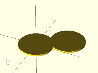
Two cylinders
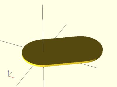
Convex hull of two cylinders
Displays the convex hull of child nodes.
Usage example:


