Customer segmentation – LifeCycle Grids, CLV and CAC with R

We studied a very powerful approach for customer segmentation in the previous post, which is based on the customer’s lifecycle. We used two metrics: frequency and recency. It is also possible and very helpful to add monetary value to our segmentation. If you havecustomer acquisition cost (CAC) and customer lifetime value (CLV), you can easily add these data to the calculations.

We will create the same data sample as in the previous post, but with two added data frames:

• cac, our expenses for each customer acquisition,
• gr.margin, gross margin of each product.

# loading libraries
library (dplyr)
library (reshape2)
library (ggplot2)

# creating data sample
set.seed (10)
data <- data.frame (orderId= sample ( c (1:1000), 5000, replace= TRUE ),
product= sample ( c ( 'NULL' , 'a' , 'b' , 'c' ), 5000, replace= TRUE ,
prob= c (0.15, 0.65, 0.3, 0.15)))
order <- data.frame (orderId= c (1:1000),
clientId= sample ( c (1:300), 1000, replace= TRUE ))
gender <- data.frame (clientId= c (1:300),
gender= sample ( c ( 'male' , 'female' ), 300, replace= TRUE , prob= c (0.40, 0.60)))
date <- data.frame (orderId= c (1:1000),
orderdate= sample ((1:100), 1000, replace= TRUE ))
orders <- merge (data, order, by= 'orderId' )
orders <- merge (orders, gender, by= 'clientId' )
orders <- merge (orders, date, by= 'orderId' )
orders <- orders[orders$product!= 'NULL' , ]
orders$orderdate <- as.Date (orders$orderdate, origin= "2012-01-01" )

# creating data frames with CAC and Gross margin
cac <- data.frame (clientId= unique (orders$clientId), cac= sample ( c (10:15), 289, replace= TRUE ))
gr.margin <- data.frame (product= c ( 'a' , 'b' , 'c' ), grossmarg= c (1, 2, 3))

rm (data, date, order, gender)

Next, we will calculate CLV to date (actual amount that we earned) using gross margin values and orders of the products. We will use the following code:

# reporting date
today <- as.Date ( '2012-04-11' , format= '%Y-%m-%d' )

# calculating customer lifetime value
orders <- merge (orders, gr.margin, by= 'product' )

clv <- orders %>%
group_by (clientId) %>%
summarise (clv= sum (grossmarg))

# processing data
orders <- dcast (orders, orderId + clientId + gender + orderdate ~ product, value.var= 'product' , fun.aggregate=length)

orders <- orders %>%
group_by (clientId) %>%
mutate (frequency= n (),
recency= as.numeric (today-orderdate)) %>%
filter (orderdate== max (orderdate)) %>%
filter (orderId== max (orderId))

orders.segm <- orders %>%
mutate (segm.freq= ifelse ( between (frequency, 1, 1), '1' ,
ifelse ( between (frequency, 2, 2), '2' ,
ifelse ( between (frequency, 3, 3), '3' ,
ifelse ( between (frequency, 4, 4), '4' ,
ifelse ( between (frequency, 5, 5), '5' , '>5' )))))) %>%
mutate (segm.rec= ifelse ( between (recency, 0, 6), '0-6 days' ,
ifelse ( between (recency, 7, 13), '7-13 days' ,
ifelse ( between (recency, 14, 19), '14-19 days' ,
ifelse ( between (recency, 20, 45), '20-45 days' ,
ifelse ( between (recency, 46, 80), '46-80 days' , '>80 days' )))))) %>%
# creating last cart feature
mutate (cart= paste ( ifelse (a!=0, 'a' , '' ),
ifelse (b!=0, 'b' , '' ),
ifelse (c!=0, 'c' , '' ), sep= '' )) %>%
arrange (clientId)

# defining order of boundaries
orders.segm$segm.freq <- factor (orders.segm$segm.freq, levels= c ( '>5' , '5' , '4' , '3' , '2' , '1' ))
orders.segm$segm.rec <- factor (orders.segm$segm.rec, levels= c ( '>80 days' , '46-80 days' , '20-45 days' , '14-19 days' , '7-13 days' , '0-6 days' ))

Note: if you prefer to use potential/expected/predicted CLV or total CLV (sum of CLV to date and potential CLV) you can adapt this code or find the example in the next post.

In addition, we need to merge orders.segm with the CAC and CLV data, and combine the data with the segments. We will calculate total CAC and CLV to date, as well as their average with the following code:

orders.segm <- merge (orders.segm, cac, by= 'clientId' )
orders.segm <- merge (orders.segm, clv, by= 'clientId' )

lcg.clv <- orders.segm %>%
group_by (segm.rec, segm.freq) %>%
summarise (quantity= n (),
# calculating cumulative CAC and CLV
cac= sum (cac),
clv= sum (clv)) %>%
ungroup () %>%
# calculating CAC and CLV per client
mutate (cac1= round (cac/quantity, 2),
clv1= round (clv/quantity, 2))

lcg.clv <- melt (lcg.clv, id.vars= c ( 'segm.rec' , 'segm.freq' , 'quantity' ))

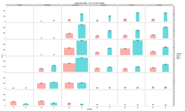
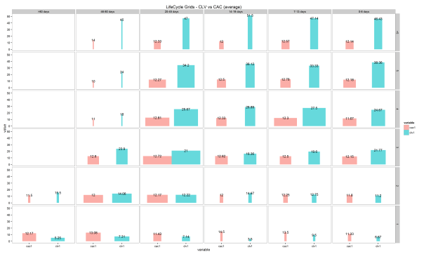
Ok, let’s plot two charts: the first one representing the totals and the second one representing the averages:

ggplot (lcg.clv[lcg.clv$variable % in % c ( 'clv' , 'cac' ), ], aes (x=variable, y=value, fill=variable)) +
theme_bw () +
theme (panel.grid = element_blank ())+
geom_bar (stat= 'identity' , alpha=0.6, aes (width=quantity/ max (quantity))) +
geom_text ( aes (y=value, label=value), size=4) +
facet_grid (segm.freq ~ segm.rec) +
ggtitle ( "LifeCycle Grids - CLV vs CAC (total)" )
ggplot (lcg.clv[lcg.clv$variable % in % c ( 'clv1' , 'cac1' ), ], aes (x=variable, y=value, fill=variable)) +
theme_bw () +
theme (panel.grid = element_blank ())+
geom_bar (stat= 'identity' , alpha=0.6, aes (width=quantity/ max (quantity))) +
geom_text ( aes (y=value, label=value), size=4) +
facet_grid (segm.freq ~ segm.rec) +
ggtitle ( "LifeCycle Grids - CLV vs CAC (average)" )

You can find in the grid that the width of bars depends on the number of customers. I think these visualizations are very helpful. You can see the difference between CLV to dateand CAC and make decisions about on paid campaigns or initiatives like:

• does it make sense to spend extra money to reactivate some customers (e.g. those who are in the “1 order / >80 days“ grid or those who are in the “>5 orders / 20-45 days“ grid)?,
• how much money is appropriate to spend?,
• and so on.

Therefore, we have got a very interesting visualization. We can analyze and make decisions based on the three customer lifecycle metrics: recency, frequency andmonetary value.

Thank you for reading this!

 

转自：http://analyzecore.com/2015/02/19/customer-segmentation-lifecycle-grids-clv-and-cac-with-r/