Level set method: Explanation
Here the basics of the level set method is explained, this is not an advanced tutorial. For quite some time, I was afraid of the level set method. I am still not sure why I first got scared. The level set method is just plain easy to understand: there is a surface, it intersects a plane, that gives us a contour and that's it. With image segmentation, the surface is updated with forces derived from the image. In this document, I follow this path: what is the problem, what was done to solve it and where the limitation was, and then the miracle solution with some pretty pictures.
Tracking interfaces
First, let us imagine water falling from the top of a hill. The goal is to track the water front while it's moving down the hill. The figure below shows a map of a V-shaped water fall with water motion shown in red.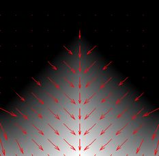 |
The question now is where is the water front at a given time t ?
Explicit contours
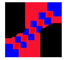
One way is to keep track of a few points, advance them in the normal direction to the front (the red arrows), and guess where the front ends up. The figure below shows a step of this technique.
Evolving explicitly the front with a set of points may sound a good solution, but there are a couple of drawbacks that may want you to not use this technique.
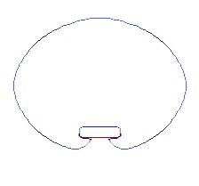
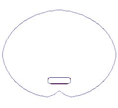
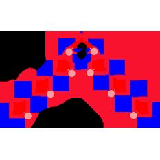
With our last example of a V-shaped propagating front, corners can end up in an unknown state. The figure below illustrates such a state after one iteration.
Also, if the front is expanding, the initial set of points may not be sufficient enough to define the evolving front. Points should be inserted or removed in the front when it is collapsing, and distance between points should be kept small enough for a smooth front. Such a mechanism could be troublesome during implementation.
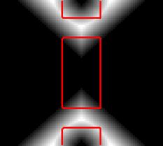
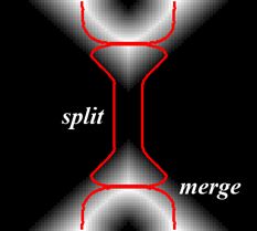
Topology change requires further care during implementation (eg. split and merge of fronts). In our hill example, let us now imagine valleys and water moving from the top down into the valleys. The figure below illustrates such a scenario. The challenge is how to insert or remove points during a topology change.
|
Tracking the front with explicit contours is intuitive but can get troublesome during implementation.
Implicit contours
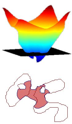
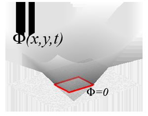
The idea of evolving a surface () instead of a front (C) was proposed, and the front is defined to be all points where the surface has no height (![]() ). The front is then defined implicitly as the zero level set
). The front is then defined implicitly as the zero level set ![]() . The figure below shows how the contour is extracted from the evolving surface.
. The figure below shows how the contour is extracted from the evolving surface.
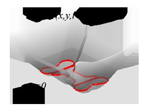
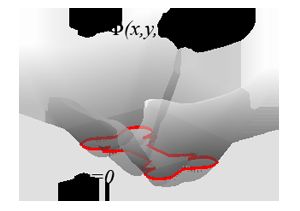
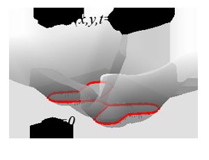
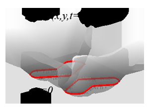
When the surface evolves, cups can appear, they can later narrow, or disappear. The zero level set shows contours spliting and merging as illustrated in the figure below where the plane at z=0 represents the map of our valley. The intersection of the surface with the plane creates the implicit contour. Merging and spliting are here handled naturally by the surface motion.
|
No extra care is needed for topology change. This looks like an interesting idea, the question is now: what is the function ?
Level set equation
Let us look at the math behind this idea. A point ![]() belonging to a front evolves over time so that
belonging to a front evolves over time so that ![]() is its position over time. At any time t, for each point
is its position over time. At any time t, for each point ![]() on the front the surface has by definition no height, thus:
on the front the surface has by definition no height, thus:
The question still remains: what is the function ![]() ? It can actually be anything we want as long as its zero level set gives us the contour. For example, a previous figure (
? It can actually be anything we want as long as its zero level set gives us the contour. For example, a previous figure () showed an initial squared contour. The surface height is equal to the distance from (x,y) to the closest point on the contour, so that
![]() , with distance d positive outside the contour, and d negative inside it. So the initial can actually be any arbitrary function as long as its zero level set matches the initial contour
, with distance d positive outside the contour, and d negative inside it. So the initial can actually be any arbitrary function as long as its zero level set matches the initial contour
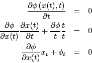
Given an initial at t=0, it would be possible to know at any time t with the motion equation![]() . For that, the chain rule gives us:
. For that, the chain rule gives us:
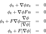
Here, recall that ![]() . Also, the speed
. Also, the speed ![]() is given by a force F normal to the surface, so
is given by a force F normal to the surface, so![]() where
where ![]() . The previous motion equation can be rewriten with:
. The previous motion equation can be rewriten with:
This last equation defines the motion of . Given at time t=0, and its motion over time, it is now possible to know ![]() at any time t by evolving the initial
at any time t by evolving the initial ![]() over time. This answers our initial question, we now know what is.
over time. This answers our initial question, we now know what is.
An interesting feature that comes with is that it is possible to get the surface curvature with:
This could be useful to control the front smoothness.
Implementation
In the computer world, images have pixels and functions need to be discretized. That means ![]() will be evaluated at pixel (i,j) by
will be evaluated at pixel (i,j) by ![]() . The gradient will be evaluated by a finite difference scheme, for example with:
. The gradient will be evaluated by a finite difference scheme, for example with:
Here, ![]() or
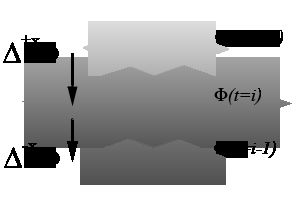
or ![]() is the left or the right side finite difference for a given point. This is illustrated in the figure below. The gradient is computed differently depending on the front direction and a finite difference scheme takes account of that.
is the left or the right side finite difference for a given point. This is illustrated in the figure below. The gradient is computed differently depending on the front direction and a finite difference scheme takes account of that.
The previous motion equation now becomes:
From there, updating the surface ![]() is done with:
is done with:
When computing the curvature, it depends only on the surface , so central differences can be used. They are:
The curvature is then computed numerically with:
To keep a front smooth, high curvature should be penalized. That means, rather than decreasing in order to have the zero level set expanding, high curvature will reverse the front motion. Updating ![]() with the curvature could be:
with the curvature could be:
Results
Given an initial arbitrary , for example the distance transform of an initial contour, and a numerical scheme for the motion equation ![]() , it is possible to show some examples of contour evolution.
, it is possible to show some examples of contour evolution.
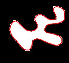
First a simple example of a drop of water exanding (F=1 everywhere) with an obstacle on its path (where F=0). The water front should be stopped by the obstacle and later be perturbed by the obstacle. This is shown in the figures below.
|
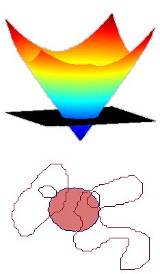
Then, a slightly more complex form illustrated below. The initial contour is still a circle, and the forces applied to it is positive (F=1) inside a form, and it is negative (F=-1) outside it. The contour should then be attracted into the form. Also notice the front split between the two regions. Here, the surface is also shown to explain how this split is formed.
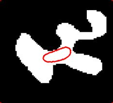
After having shown how constant forces act on , the next example shows a shape collapsing under its curvature. Here the force is equal to the curvature ![]() of the surface .
of the surface .
|
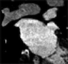
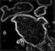
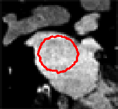
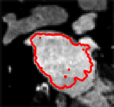
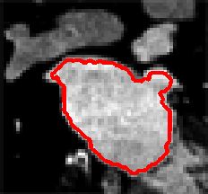
Now the fun begins with real pictures. Instead of using constant positive or negative forces, with or without curvature, the force is derived from an image. We can think of a contour stopped at the edges of an object. The force should then be high inside the object (we want the curve expanding inside an object), and it should be low close to the edges (we want the curve to stop at the edges). The gradient of an image shows where the edges are.
The force to be used could be the inverse of the previous gradient image ![]() , or it could be the gaussian of it:
, or it could be the gaussian of it:
Here ![]() or
or ![]() are parameters controlling how penalizing the edges should be. Below is an evolving contour using the inverse of the gradient image.
are parameters controlling how penalizing the edges should be. Below is an evolving contour using the inverse of the gradient image.
|
At this point, you should at least understand that level set method is all about evolving a surface instead of the real contour. That makes the beauty of this method. Level sets have applications in many fields. See google for further reading.
Bibliography
- 1
- Osher S., Sethian J.A., Fronts Propagating with Curvature-Dependent Speed: Algorithms Based on Hamilton-Jacobi Formulations (Journal of Computational Physics, 79(1), page 12-49, 1988).
- 2
- Kass M., Witkin A., Terzopoulos D., Snakes - Active Contour Models (International Journal of Computer Vision, 1(4), page 321-331, 1987)
![\begin{eqnarray*}\nabla^{+x}(i,j) = max\left[0,\Delta^{-x}\phi(i,j)\right]^2 + ......2 + min\left[0,\Delta^{-x}\phi(i,j)\right]^2, \textrm{when} F<0.\end{eqnarray*}](http://img.e-com-net.com/image/info5/4030da49f09b4c41a7155214c7ef6e17.png)
