UFLDL——Exercise: Sparse Autoencoder 稀疏自动编码

实验要求可以参考deeplearning的tutorial，Exercise:Sparse Autoencoder。稀疏自动编码的原理可以参照之前的博文，神经网络， 稀疏自动编码   。

1. 神经网络结构：

实验是实现三层的稀疏自动编码神经网络，神经网络结构包括输入层64个neuron，隐含层25个neuron（都不包括bias结点），输出层和输入层相同的neuron的个数。

2. 训练数据：

实验中的原始数据是10副512×512大小的灰度图像，存储在“IMAGES.mat”文件中。下图是其中的一张图像。

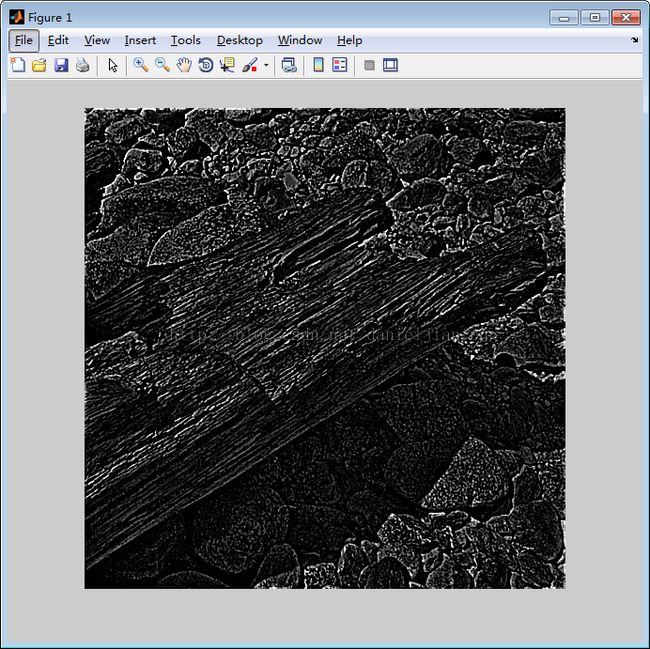
我们随机中10副图像中挑选一个，然后再从该图像中随机的选一个8*8的图像patch，得到的这个patch作为一个训练数据，重复这个随机过程10000，最后得到10000数据组成的训练集，存储在64×10000 的矩阵，每一列代表一个数据。

 

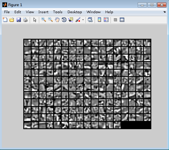
下图是总10000个数据中随机挑选出100个进行显示。

3. 损失函数（loss function）

稀疏自动编码的损失函数由三部分组成，公式如下：

4. 偏导数（partial derivatives）

偏导数的计算是通过BP算法，需要注意是，由于在实验中使用的是batch的优化方法，所以偏导数计算的时候对所有样本的偏导数做了一个求和操作。

 

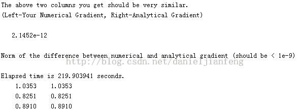
5.梯度检验（Gradient checking）

有网友说他们在自己的电脑上跑Gradient checking这步的时候用了1个多小时，但不知道是不是我的电脑配置比较高，我才跑了不到4分钟。

6. 用L-BFGS算法进行训练

因为我们已经有了损失函数和相应参数的偏导数，所以和直接用成熟的L-BFGS算法的包，最后算法到底最大迭代次数400的时候，停止迭代。

7. 实验结果：

下图显示的是第一层到第二层的参数，由于输入层为64个neuron，隐含层为25个neuron，所以下面共有25个patch，每一个patch大小为8*8.

源代码下载

sampleIMAGES.m

function patches = sampleIMAGES()
% sampleIMAGES
% Returns 10000 patches for training

load IMAGES;    % load images from disk 

patchsize = 8;  % we'll use 8x8 patches 
numpatches = 10000;

% Initialize patches with zeros.  Your code will fill in this matrix--one
% column per patch, 10000 columns. 
patches = zeros(patchsize*patchsize, numpatches);

%% ---------- YOUR CODE HERE --------------------------------------
%  Instructions: Fill in the variable called "patches" using data 
%  from IMAGES.  
%  
%  IMAGES is a 3D array containing 10 images
%  For instance, IMAGES(:,:,6) is a 512x512 array containing the 6th image,
%  and you can type "imagesc(IMAGES(:,:,6)), colormap gray;" to visualize
%  it. (The contrast on these images look a bit off because they have
%  been preprocessed using using "whitening."  See the lecture notes for
%  more details.) As a second example, IMAGES(21:30,21:30,1) is an image
%  patch corresponding to the pixels in the block (21,21) to (30,30) of
%  Image 1

for i = 1:numpatches
    x = ceil(rand(1)*505);
    y = ceil(rand(1)*505);
    z = ceil(rand(1)*10);
    patch = IMAGES(x : x+patchsize-1, y : y+patchsize-1, z);
    patches(:,i) = patch(:);    
end



%% ---------------------------------------------------------------
% For the autoencoder to work well we need to normalize the data
% Specifically, since the output of the network is bounded between [0,1]
% (due to the sigmoid activation function), we have to make sure 
% the range of pixel values is also bounded between [0,1]
patches = normalizeData(patches);

end


%% ---------------------------------------------------------------
function patches = normalizeData(patches)

% Squash data to [0.1, 0.9] since we use sigmoid as the activation
% function in the output layer

% Remove DC (mean of images). 
patches = bsxfun(@minus, patches, mean(patches));

% Truncate to +/-3 standard deviations and scale to -1 to 1
pstd = 3 * std(patches(:));
patches = max(min(patches, pstd), -pstd) / pstd;

% Rescale from [-1,1] to [0.1,0.9]
patches = (patches + 1) * 0.4 + 0.1;

end

sparseAutoencoderCost.m

function [cost,grad] = sparseAutoencoderCost(theta, visibleSize, hiddenSize, ...
                                             lambda, sparsityParam, beta, data)

% visibleSize: the number of input units (probably 64) 
% hiddenSize: the number of hidden units (probably 25) 
% lambda: weight decay parameter
% sparsityParam: The desired average activation for the hidden units (denoted in the lecture
%                           notes by the greek alphabet rho, which looks like a lower-case "p").
% beta: weight of sparsity penalty term
% data: Our 64x10000 matrix containing the training data.  So, data(:,i) is the i-th training example. 
  
% The input theta is a vector (because minFunc expects the parameters to be a vector). 
% We first convert theta to the (W1, W2, b1, b2) matrix/vector format, so that this 
% follows the notation convention of the lecture notes. 

W1 = reshape(theta(1:hiddenSize*visibleSize), hiddenSize, visibleSize);
W2 = reshape(theta(hiddenSize*visibleSize+1:2*hiddenSize*visibleSize), visibleSize, hiddenSize);
b1 = theta(2*hiddenSize*visibleSize+1:2*hiddenSize*visibleSize+hiddenSize);
b2 = theta(2*hiddenSize*visibleSize+hiddenSize+1:end);

% Cost and gradient variables (your code needs to compute these values). 
% Here, we initialize them to zeros. 
cost = 0;
W1grad = zeros(size(W1)); 
W2grad = zeros(size(W2));
b1grad = zeros(size(b1)); 
b2grad = zeros(size(b2));

%% ---------- YOUR CODE HERE --------------------------------------
%  Instructions: Compute the cost/optimization objective J_sparse(W,b) for the Sparse Autoencoder,
%                and the corresponding gradients W1grad, W2grad, b1grad, b2grad.
%
% W1grad, W2grad, b1grad and b2grad should be computed using backpropagation.
% Note that W1grad has the same dimensions as W1, b1grad has the same dimensions
% as b1, etc.  Your code should set W1grad to be the partial derivative of J_sparse(W,b) with
% respect to W1.  I.e., W1grad(i,j) should be the partial derivative of J_sparse(W,b) 
% with respect to the input parameter W1(i,j).  Thus, W1grad should be equal to the term 
% [(1/m) \Delta W^{(1)} + \lambda W^{(1)}] in the last block of pseudo-code in Section 2.2 
% of the lecture notes (and similarly for W2grad, b1grad, b2grad).
% 
% Stated differently, if we were using batch gradient descent to optimize the parameters,
% the gradient descent update to W1 would be W1 := W1 - alpha * W1grad, and similarly for W2, b1, b2. 
% 


% data = [ones(1,size(data,2)); data];
[n m] = size(data);

z2 = W1* data + repmat(b1,1,m);
a2 = sigmoid(z2);
z3 = W2 * a2 + repmat(b2,1,m); 
a3 = sigmoid(z3);

phat = mean(a2,2);
p = repmat(sparsityParam, size(phat));
sparse = p .* log(p ./ phat) + (1-p) .* log((1-p) ./ (1-phat));

%J = trace((data - a3)' * (data - a3)) / (size(data,2)*2);
J = sum(sum((a3-data).^2)) / (m*2);

regu = (W1(:)'*W1(:) + W2(:)'*W2(:))/2;

cost = J + lambda*regu + beta * sum(sparse);



delta3 = -1* (data-a3).*a3.*(1-a3);
delta2 = (W2'*delta3+beta*repmat(-p./phat+(1-p)./(1-phat),1,size(data,2))).*a2.*(1-a2); 


W2grad = delta3*a2'/m;  
b2grad = mean(delta3,2);  
W1grad = delta2*data'/m;  
b1grad = mean(delta2,2); 

W2grad = W2grad + lambda*W2;  
W1grad = W1grad + lambda*W1;  


%-------------------------------------------------------------------
% After computing the cost and gradient, we will convert the gradients back
% to a vector format (suitable for minFunc).  Specifically, we will unroll
% your gradient matrices into a vector.

grad = [W1grad(:) ; W2grad(:) ; b1grad(:) ; b2grad(:)];

end

%-------------------------------------------------------------------
% Here's an implementation of the sigmoid function, which you may find useful
% in your computation of the costs and the gradients.  This inputs a (row or
% column) vector (say (z1, z2, z3)) and returns (f(z1), f(z2), f(z3)). 

function sigm = sigmoid(x)
  
    sigm = 1 ./ (1 + exp(-x));
end