图像频域变换及应用
图像频域变换及应用
1.名词解释:
(1)空间域:英文:spatial domain。释文:又称图像空间(imagespace)。由图像像元组成的空间。在图像空间中以长度(距离)为自变量直接对像元值进行处理称为空间域处理。
(2)频率域:英文:spatial frequency domain。释文:以空间频率(即波数)为自变量描述图像的特征,可以将一幅图像像元值在空间上的变化分解为具有不同振幅、空间频率和相位的简振函数的线性叠加,图像中各种空间频率成分的组成和分布称为空间频谱。这种对图像的空间频率特征进行分解、处理和分析称为空间频率域处理或波数域处理。
(3)二者关系:
空间域与频率域可互相转换。在空间频率域中可以引用已经很成熟的频率域技术,处理的一般步骤为:
①对图像施行二维离散傅立叶变换或小波变换,将图像由图像空间转换到频域空间。
②在频率域中对图像的频谱作分析处理,以改变图像的频率特征。即设计不同的数字滤波器,对图像的频谱进行滤波。频率域处理主要用于与图像空间频率有关的处理中。如图像恢复、图像重建、辐射变换、边缘增强、图像锐化、图像平滑、噪声压制、频谱分析、纹理分析等处理和分析中。须注意,空间频率(波数)的单位为米 -l或(毫米)-1等。
2.应用:
(1)对test 目录下的图像:
查看不同图像的傅立叶变换的图像;
查看不同图像的DCT(离散余弦)变换;
(2)对变换后的图像使用空间域图像增强的方法增强效果;
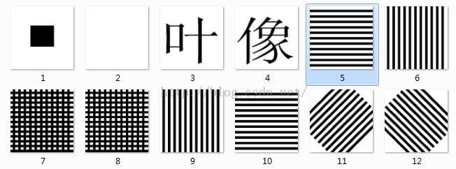
比较5.bmp和10.bmp、6.bmp和9.bmp频率域图像的不同;
(3)使用低通滤波器,查看结果;
(4)使用高通滤波器,查看结果。
3.常用函数:
(1)频率域处理函数:
① 傅里叶变换fft2();
② 傅里叶逆变换ifft2();
③ 离散余弦变换dct2();
④ 频域滤波函数:dftfilt(f,H)。
查看不同图像的DCT(离散余弦)变换;
(3)使用低通滤波器,查看结果;
(4)使用高通滤波器,查看结果。
3.常用函数:
(1)频率域处理函数:
① 傅里叶变换fft2();
② 傅里叶逆变换ifft2();
③ 离散余弦变换dct2();
④ 频域滤波函数:dftfilt(f,H)。
(2)空间域图像增强
① 线性变换 transfor();
② 指数变换 exp();
③ 对数变换 log();
④ 幂次变换 power();
⑤ 查看直方图 imhist();
⑥ 使用直方图均衡Histeq();
⑦ 使用平滑滤波器(imfilter实现函数滤波);
⑧ 使用锐化滤波器。
(3)傅里叶变换过程:
 F = fft2(f)
     S = abs(F); 傅里叶谱
 Fc = fftshift(F); 象限变换
 S2 = log(1+abs(Fc)); 对数变换
 Im2uint8(mat2gray(g))
4.matlab源码:
全部文件截图如下:
(1) adjusttoday.m
function adjusttoday(strFileName);

I = imread(strFileName);
J = imadjust(I,[0.3 0.7],[0.1 0.9],[]);

J = uint8(I);

imshow(J);
(2) dcttoday.m
function dcttoday(strFileName);

RGB = imread(strFileName);
I = rgb2gray(RGB);
J = dct2(I);
figure, imshow(log(abs(J)), []);

colormap(jet(64));
colorbar;
(3) dftfilt.m
function g = dftfilt(f, H)
%DFTFILT Performs frequency domain filtering.
%   G = DFTFILT(F, H) filters F in the frequency domain using the
%   filter transfer function H. The output, G, is the filtered
%   image, which has the same size as F.  DFTFILT automatically pads
%   F to be the same size as H.  Function PADDEDSIZE can be used to
%   determine an appropriate size for H.
%
%   DFTFILT assumes that F is real and that H is a real, uncentered
%   circularly-symmetric filter function.

%   Copyright 2002-2004 R. C. Gonzalez, R. E. Woods, & S. L. Eddins
%   Digital Image Processing Using MATLAB, Prentice-Hall, 2004
%   $Revision: 1.5 $  $Date: 2003/08/25 14:28:22 $

% Obtain the FFT of the padded input.
F = fft2(f, size(H, 1), size(H, 2));

% Perform filtering.
g = real(ifft2(H.*F));

% Crop to original size.
g = g(1:size(f, 1), 1:size(f, 2));
(4) FFTShow.m
function FFTShow(strFilename);

I=imread(strFilename);
I=rgb2gray(I);
figure,imshow(I);

str=strcat(strFilename, 'FFT');
F = fft2(I);
 F2 = log(abs(F));
figure,imshow(F,[-1 5],'notruesize'),Title(str); colormap(jet); colorbar

D=dct2(I);
 D2 = log(abs(D));
figure,imshow(D2,[-1 5],'notruesize');  %colormap(jet); colorbar
(5) ffttoday.m
function ffttoday(strFileName);

I = imread(strFileName);
F = fft2(I);
S = abs(F);
Fc = fftshift(F);
S2 = log(1+abs(Fc));
outcome = Im2uint8(mat2gray(S2));

subplot(221); imshow(I);
subplot(222); imshow(F);
subplot(223); imshow(S);
subplot(224); imshow(Fc);

figure, imshow(S2);
figure, imshow(outcome);
(6) Freq.m
function FFTShow(strFilename);

I=imread(strFilename);
%   I=rgb2gray(I);
figure,imshow(I);

F = fft2(I);
 F2 = log(abs(F));
figure,imshow(F2,[-1 5],'notruesize'),Title(strFilename+ 'FFT');% colormap(jet); colorbar

D=dct2(I);
% D2 = log(abs(D));
figure,imshow(D,[-1 5],'notruesize'); % colormap(jet); colorbar
(7) hpfilter.m
function H = hpfilter(type, M, N, D0, n)
%HPFILTER Computes frequency domain highpass filters.
%   H = HPFILTER(TYPE, M, N, D0, n) creates the transfer function of
%   a highpass filter, H, of the specified TYPE and size (M-by-N).
%   Valid values for TYPE, D0, and n are:
%
%   'ideal'    Ideal highpass filter with cutoff frequency D0.  n
%              need not be supplied. D0 must be positive.
%
%   'btw'      Butterworth highpass filter of order n, and cutoff
%              D0.  The default value for n is 1.0. D0 must be
%              positive.
%
%   'gaussian' Gaussian highpass filter with cutoff (standard
%              deviation) D0. n need not be supplied. D0 must be
%              positive.

%   Copyright 2002-2004 R. C. Gonzalez, R. E. Woods, & S. L. Eddins
%   Digital Image Processing Using MATLAB, Prentice-Hall, 2004
%   $Revision: 1.4 $  $Date: 2003/08/25 14:28:22 $

% The transfer function Hhp of a highpass filter is 1 - Hlp,
% where Hlp is the transfer function of the corresponding lowpass
% filter.  Thus, we can use function lpfilter to generate highpass
% filters.

if nargin == 4
   n = 1; % Default value of n.
end

% Generate highpass filter.
Hlp = lpfilter(type, M, N, D0, n);
H = 1 - Hlp;
(8) lpfilter.m
function H = lpfilter(type, M, N, D0, n)
%LPFILTER Computes frequency domain lowpass filters.
%   H = LPFILTER(TYPE, M, N, D0, n) creates the transfer function of
%   a lowpass filter, H, of the specified TYPE and size (M-by-N). To
%   view the filter as an image or mesh plot, it should be centered
%   using H = fftshift(H).
%
%   Valid values for TYPE, D0, and n are:
%
%   'ideal'    Ideal lowpass filter with cutoff frequency D0. n need
%              not be supplied.  D0 must be positive.
%
%   'btw'      Butterworth lowpass filter of order n, and cutoff
%              D0.  The default value for n is 1.0.  D0 must be
%              positive.
%
%   'gaussian' Gaussian lowpass filter with cutoff (standard
%              deviation) D0.  n need not be supplied.  D0 must be
%              positive.

%   Copyright 2002-2004 R. C. Gonzalez, R. E. Woods, & S. L. Eddins
%   Digital Image Processing Using MATLAB, Prentice-Hall, 2004
%   $Revision: 1.7 $  $Date: 2003/10/13 00:46:25 $

% Use function dftuv to set up the meshgrid arrays needed for
% computing the required distances.
%[U, V] = dftuv(M, N);
U = M;V= N;
% Compute the distances D(U, V).
D = sqrt(U.^2 + V.^2);

% Begin filter computations.
switch type
case 'ideal'
   H = double(D = D0);
case 'btw'
   if nargin == 4
      n = 1;
   end
   H = 1./(1 + (D./D0).^(2*n));
case 'gaussian'
   H = exp(-(D.^2)./(2*(D0^2)));
otherwise
   error('Unknown filter type.')
end
(9) paddedsize.m
function PQ = paddedsize(AB, CD, PARAM)
%PADDEDSIZE Computes padded sizes useful for FFT-based filtering.
%   PQ = PADDEDSIZE(AB), where AB is a two-element size vector,
%   computes the two-element size vector PQ = 2*AB.
%
%   PQ = PADDEDSIZE(AB, 'PWR2') computes the vector PQ such that
%   PQ(1) = PQ(2) = 2^nextpow2(2*m), where m is MAX(AB).
%
%   PQ = PADDEDSIZE(AB, CD), where AB and CD are two-element size
%   vectors, computes the two-element size vector PQ.  The elements
%   of PQ are the smallest even integers greater than or equal to
%   AB + CD -1.
%
%   PQ = PADDEDSIZE(AB, CD, 'PWR2') computes the vector PQ such that
%   PQ(1) = PQ(2) = 2^nextpow2(2*m), where m is MAX([AB CD]).

if nargin == 1
   PQ = 2*AB;
elseif nargin == 2 & ~ischar(CD)
   PQ = AB + CD - 1;
   PQ = 2 * ceil(PQ / 2);
elseif nargin == 2
   m = max(AB); % Maximum dimension.

   % Find power-of-2 at least twice m.
   P = 2^nextpow2(2*m);
   PQ = [P, P];
elseif nargin == 3
   m = max([AB CD]); %Maximum dimension.
   P = 2^nextpow2(2*m);
   PQ = [P, P];
else
   error('Wrong number of inputs.')
end
(10) 测试用的图片:test