原网站http://www.coin-or.org/Ipopt/documentation/node37.html
Triplet Format for Sparse Matrices
I
POPT
was designed for optimizing large sparse nonlinear programs. Because of problem sparsity, the required matrices (like the constraints Jacobian or Lagrangian Hessian) are not stored as dense matrices, but rather in a sparse matrix format. For the tutorials in this document, we use the triplet format. Consider the matrix
A standard dense matrix representation would need to store floating point numbers, where many entries would be zero. In triplet format, however, only the nonzero entries are stored. The triplet format records the row number, the column number, and the value of all nonzero entries in the matrix. For the matrix above, this means storing  integers for the rows,
  integers for the columns, and
  floating point numbers for the values. While this does not seem like a huge space saving over the
  floating point numbers stored in the dense representation, for larger matrices, the space savings are very dramatic24.
The parameter index_style in get_nlp_info tells IPOPT if you prefer to use C style indexing (0-based, i.e., starting the counting at 0) for the row and column indices or Fortran style (1-based). Tables 3 and 4 below show the triplet format for both indexing styles, using the example matrix (14).
Table 3: Triplet Format of Matrix ( 14) with index_style=FORTRAN_STYLE
| row |
col |
value |
| iRow[0] = 1 |
jCol[0] = 1 |
values[0] = 1.1 |
| iRow[1] = 1 |
jCol[1] = 7 |
values[1] = 0.5 |
| iRow[2] = 2 |
jCol[2] = 2 |
values[2] = 1.9 |
| iRow[3] = 2 |
jCol[3] = 7 |
values[3] = 0.5 |
| iRow[4] = 3 |
jCol[4] = 3 |
values[4] = 2.6 |
| iRow[5] = 3 |
jCol[5] = 7 |
values[5] = 0.5 |
| iRow[6] = 4 |
jCol[6] = 3 |
values[6] = 7.8 |
| iRow[7] = 4 |
jCol[7] = 4 |
values[7] = 0.6 |
| iRow[8] = 5 |
jCol[8] = 4 |
values[8] = 1.5 |
| iRow[9] = 5 |
jCol[9] = 5 |
values[9] = 2.7 |
| iRow[10] = 6 |
jCol[10] = 1 |
values[10] = 1.6 |
| iRow[11] = 6 |
jCol[11] = 5 |
values[11] = 0.4 |
| iRow[12] = 7 |
jCol[12] = 6 |
values[12] = 0.9 |
| iRow[13] = 7 |
jCol[13] = 7 |
values[13] = 1.7 |
|
Table 4: Triplet Format of Matrix ( 14) with index_style=C_STYLE
| row |
col |
value |
| iRow[0] = 0 |
jCol[0] = 0 |
values[0] = 1.1 |
| iRow[1] = 0 |
jCol[1] = 6 |
values[1] = 0.5 |
| iRow[2] = 1 |
jCol[2] = 1 |
values[2] = 1.9 |
| iRow[3] = 1 |
jCol[3] = 6 |
values[3] = 0.5 |
| iRow[4] = 2 |
jCol[4] = 2 |
values[4] = 2.6 |
| iRow[5] = 2 |
jCol[5] = 6 |
values[5] = 0.5 |
| iRow[6] = 3 |
jCol[6] = 2 |
values[6] = 7.8 |
| iRow[7] = 3 |
jCol[7] = 3 |
values[7] = 0.6 |
| iRow[8] = 4 |
jCol[8] = 3 |
values[8] = 1.5 |
| iRow[9] = 4 |
jCol[9] = 4 |
values[9] = 2.7 |
| iRow[10] = 5 |
jCol[10] = 0 |
values[10] = 1.6 |
| iRow[11] = 5 |
jCol[11] = 4 |
values[11] = 0.4 |
| iRow[12] = 6 |
jCol[12] = 5 |
values[12] = 0.9 |
| iRow[13] = 6 |
jCol[13] = 6 |
values[13] = 1.7 |
|
The individual elements of the matrix can be listed in any order, and if there are multiple items for the same nonzero position, the values provided for those positions are added.
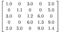
The Hessian of the Lagrangian is a symmetric matrix. In the case of a symmetric matrix, you only need to specify the lower left triangular part (or, alternatively, the upper right triangular part). For example, given the matrix,
 |
(15) |
the triplet format is shown in Tables 5
and 6
.
Table 5: Triplet Format of Matrix ( 15) with index_style=FORTRAN_STYLE
| row |
col |
value |
| iRow[0] = 1 |
jCol[0] = 1 |
values[0] = 1.0 |
| iRow[1] = 2 |
jCol[1] = 1 |
values[1] = 1.1 |
| iRow[2] = 3 |
jCol[2] = 1 |
values[2] = 3.0 |
| iRow[3] = 3 |
jCol[3] = 3 |
values[3] = 1.2 |
| iRow[4] = 4 |
jCol[4] = 3 |
values[4] = 6.0 |
| iRow[5] = 4 |
jCol[5] = 4 |
values[5] = 1.3 |
| iRow[6] = 5 |
jCol[6] = 1 |
values[6] = 2.0 |
| iRow[7] = 5 |
jCol[7] = 2 |
values[7] = 5.0 |
| iRow[8] = 5 |
jCol[8] = 4 |
values[8] = 9.0 |
| iRow[9] = 5 |
jCol[9] = 5 |
values[9] = 1.4 |
|
Table 6: Triplet Format of Matrix ( 15) with index_style=C_STYLE
| row |
col |
value |
| iRow[0] = 0 |
jCol[0] = 0 |
values[0] = 1.0 |
| iRow[1] = 1 |
jCol[1] = 0 |
values[1] = 1.1 |
| iRow[2] = 2 |
jCol[2] = 0 |
values[2] = 3.0 |
| iRow[3] = 2 |
jCol[3] = 2 |
values[3] = 1.2 |
| iRow[4] = 3 |
jCol[4] = 2 |
values[4] = 6.0 |
| iRow[5] = 3 |
jCol[5] = 3 |
values[5] = 1.3 |
| iRow[6] = 4 |
jCol[6] = 0 |
values[6] = 2.0 |
| iRow[7] = 4 |
jCol[7] = 1 |
values[7] = 5.0 |
| iRow[8] = 4 |
jCol[8] = 3 |
values[8] = 9.0 |
| iRow[9] = 4 |
jCol[9] = 4 |
values[9] = 1.4 |
|
Footnotes
-
-
For an
 matrix, the dense representation grows with the the square of
 , while the sparse representation grows linearly in the number of nonzeros.

 Next:
Next: The Smart Pointer Implementation:
Up: Introduction to IPOPT: A
Previous: Diagnostic Tags for IPOPT
Contents
![]() integers for the rows,
integers for the rows, ![]() integers for the columns, and
integers for the columns, and ![]() floating point numbers for the values. While this does not seem like a huge space saving over the
floating point numbers for the values. While this does not seem like a huge space saving over the ![]() floating point numbers stored in the dense representation, for larger matrices, the space savings are very dramatic24.
floating point numbers stored in the dense representation, for larger matrices, the space savings are very dramatic24. matrix, the dense representation grows with the the square of
 , while the sparse representation grows linearly in the number of nonzeros.
