Machine Learning week 1 Programming Excercise

1 Octave 中的for 和 while

        for i<10,

             i = i + 1;

        end;

这样是错误的，这里的for 应该换成while。

2 Octave 中的std和mean

        函数std(x)，算出x的标准偏差。x可以是一行的matrix或者一个多行matrix，如果只有一行，那么就是算一行的标准偏差，如果有多行，就是算每一列的标准偏差。
std（x，a）也是x的标准偏差，但是a可以＝0或者1.如果是0和前面没有区别，如果是1就是最后除以n，而不是n－1.（你参考计算标准偏差的公式，一般都用除以n－1的公式。）
std (x, a, b) 这里a表示是要用n还是n－1，如果是a是0就是除以n－1，如果是1就是除以n，b这里是维数，比如说
1 2 3 4；
4 5 6 1；
如果b是1，就是按照列分，如果b是2就是按照行分，如果是三维的矩阵，b＝3就按照第三维来分数据

        M = mean(A)，如果A只有一行或者一列数据，那么计算结果为这一行或这一列的平均值，如果A是一个矩阵，那么这里默认按照列来计算平均值
        M = mean(A,dim)，dim=1 表示按照列计算，dim=2表示按照行计算

Linear regression with one variable

ex1data1.txt 下面是部分数据，第一列是城市人口数量，第二列是在此城市开分店的利润

6.1101,17.592
5.5277,9.1302
8.5186,13.662
7.0032,11.854
5.8598,6.8233
8.3829,11.886
7.4764,4.3483

主程序

%% Machine Learning Online Class - Exercise 1: Linear Regression

%  Instructions
%  ------------
% 
%  This file contains code that helps you get started on the
%  linear exercise. You will need to complete the following functions 
%  in this exericse:
%
%     warmUpExercise.m
%     plotData.m
%     gradientDescent.m
%     computeCost.m
%     gradientDescentMulti.m
%     computeCostMulti.m
%     featureNormalize.m
%     normalEqn.m
%
%  For this exercise, you will not need to change any code in this file,
%  or any other files other than those mentioned above.
%
% x refers to the population size in 10,000s
% y refers to the profit in $10,000s
%

%% Initialization
clear ; close all; clc

%% ==================== Part 1: Basic Function ====================
% Complete warmUpExercise.m 
fprintf('Running warmUpExercise ... \n');
fprintf('5x5 Identity Matrix: \n');
warmUpExercise()

fprintf('Program paused. Press enter to continue.\n');
pause;


%% ======================= Part 2: Plotting =======================
fprintf('Plotting Data ...\n')
data = load('ex1data1.txt');
X = data(:, 1); y = data(:, 2);
m = length(y); % number of training examples

% Plot Data
% Note: You have to complete the code in plotData.m
plotData(X, y);

fprintf('Program paused. Press enter to continue.\n');
pause;

%% =================== Part 3: Gradient descent ===================
fprintf('Running Gradient Descent ...\n')

X = [ones(m, 1), data(:,1)]; % Add a column of ones to x
theta = zeros(2, 1); % initialize fitting parameters

% Some gradient descent settings
iterations = 1500;
alpha = 0.01;

% compute and display initial cost
computeCost(X, y, theta)

% run gradient descent
theta = gradientDescent(X, y, theta, alpha, iterations);

% print theta to screen
fprintf('Theta found by gradient descent: ');
fprintf('%f %f \n', theta(1), theta(2));

% Plot the linear fit
hold on; % keep previous plot visible
plot(X(:,2), X*theta, '-')
legend('Training data', 'Linear regression')
hold off % don't overlay any more plots on this figure

% Predict values for population sizes of 35,000 and 70,000
predict1 = [1, 3.5] *theta;
fprintf('For population = 35,000, we predict a profit of %f\n',...
    predict1*10000);
predict2 = [1, 7] * theta;
fprintf('For population = 70,000, we predict a profit of %f\n',...
    predict2*10000);

fprintf('Program paused. Press enter to continue.\n');
pause;

%% ============= Part 4: Visualizing J(theta_0, theta_1) =============
fprintf('Visualizing J(theta_0, theta_1) ...\n')

% Grid over which we will calculate J
theta0_vals = linspace(-10, 10, 100);
theta1_vals = linspace(-1, 4, 100);

% initialize J_vals to a matrix of 0's
J_vals = zeros(length(theta0_vals), length(theta1_vals));

% Fill out J_vals
for i = 1:length(theta0_vals)
    for j = 1:length(theta1_vals)
	  t = [theta0_vals(i); theta1_vals(j)];    
	  J_vals(i,j) = computeCost(X, y, t);
    end
end


% Because of the way meshgrids work in the surf command, we need to 
% transpose J_vals before calling surf, or else the axes will be flipped
J_vals = J_vals';
% Surface plot
figure;
surf(theta0_vals, theta1_vals, J_vals)
xlabel('\theta_0'); ylabel('\theta_1');

% Contour plot
figure;
% Plot J_vals as 15 contours spaced logarithmically between 0.01 and 100
contour(theta0_vals, theta1_vals, J_vals, logspace(-2, 3, 20))
xlabel('\theta_0'); ylabel('\theta_1');
hold on;
plot(theta(1), theta(2), 'rx', 'MarkerSize', 10, 'LineWidth', 2);

1 ploting data

function plotData(x, y)
%PLOTDATA Plots the data points x and y into a new figure 
%   PLOTDATA(x,y) plots the data points and gives the figure axes labels of
%   population and profit.

% ====================== YOUR CODE HERE ======================
% Instructions: Plot the training data into a figure using the 
%               "figure" and "plot" commands. Set the axes labels using
%               the "xlabel" and "ylabel" commands. Assume the 
%               population and revenue data have been passed in
%               as the x and y arguments of this function.
%
% Hint: You can use the 'rx' option with plot to have the markers
%       appear as red crosses. Furthermore, you can make the
%       markers larger by using plot(..., 'rx', 'MarkerSize', 10);

figure; % open a new figure window

plot(x, y, 'rx', 'MarkerSize', 10);
ylabel('Profit in $10,000s');
xlabel('Population of City in 10,000s');




% ============================================================

end

2 Gradient Descent

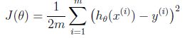
cost function

function J = computeCost(X, y, theta)
%COMPUTECOST Compute cost for linear regression
%   J = COMPUTECOST(X, y, theta) computes the cost of using theta as the
%   parameter for linear regression to fit the data points in X and y

% Initialize some useful values
m = length(y); % number of training examples

% You need to return the following variables correctly 
J = 0;

% ====================== YOUR CODE HERE ======================
% Instructions: Compute the cost of a particular choice of theta
%               You should set J to the cost.
J = sum((X * theta - y).^2)/(2*m);




% =========================================================================

end

Gradient Descent

function [theta, J_history] = gradientDescent(X, y, theta, alpha, num_iters)
%GRADIENTDESCENT Performs gradient descent to learn theta
%   theta = GRADIENTDESENT(X, y, theta, alpha, num_iters) updates theta by 
%   taking num_iters gradient steps with learning rate alpha

% Initialize some useful values
m = length(y); % number of training examples
J_history = zeros(num_iters, 1);

for iter = 1:num_iters

    % ====================== YOUR CODE HERE ======================
    % Instructions: Perform a single gradient step on the parameter vector
    %               theta. 
    %
    % Hint: While debugging, it can be useful to print out the values
    %       of the cost function (computeCost) and gradient here.
    %
    % ============================================================

    % Save the cost J in every iteration    
    theta = theta - alpha * (X' * (X * theta - y)) / m;
    J_history(iter) = computeCost(X, y, theta);

end

end

3 Visualization在主程序的part 4中通过surf方法和contour方法分别画出来cost function随着theta1和theta2的变化情况以及等高线

总结：

        1 一开始计算cost function的时候忘记1/2m的系数了，导致计算结果是一个很大的值

        2 最后一步中画surf的方法可以借鉴

        3 一个很好的习惯就是计算grandient descent的时候，跟踪J(theta)的变化，来分析cost function随着迭代的收敛情况，来决定选择合适的alpha学习速率。

        4 学习X = [ones(m, 1), data(:,1)]; % Add a column of ones to x， 其中为feature增加一列1的方法

Linear regression with multiple variables

1 dataset 第一列是房屋的面积，第二列是房屋中包含的卧室的数量，第三列是目标结果，在这里是价格

2104,3,399900
1600,3,329900
2400,3,369000
1416,2,232000
3000,4,539900
1985,4,299900
1534,3,314900
1427,3,198999

1 Feature Normalization
很容易发现，第一列和第二列数据的量级相差很大，不利于梯度下降的收敛，这里对数据进行规约，采取的方法是

（sample - mean）/ standard divation, 另外一种方案是（sample - mean）/ （max - min），这里采取第一种

使用的函数分别为mean和std计算平均值和标准差

function [X_norm, mu, sigma] = featureNormalize(X)
%FEATURENORMALIZE Normalizes the features in X 
%   FEATURENORMALIZE(X) returns a normalized version of X where
%   the mean value of each feature is 0 and the standard deviation
%   is 1. This is often a good preprocessing step to do when
%   working with learning algorithms.

% You need to set these values correctly
X_norm = X;
mu = zeros(1, size(X, 2));
sigma = zeros(1, size(X, 2));

% ====================== YOUR CODE HERE ======================
% Instructions: First, for each feature dimension, compute the mean
%               of the feature and subtract it from the dataset,
%               storing the mean value in mu. Next, compute the 
%               standard deviation of each feature and divide
%               each feature by it's standard deviation, storing
%               the standard deviation in sigma. 
%
%               Note that X is a matrix where each column is a 
%               feature and each row is an example. You need 
%               to perform the normalization separately for 
%               each feature. 
%
% Hint: You might find the 'mean' and 'std' functions useful.
%       
mu = mean(X,1);
sigma = std(X);
i = 1;
le = size(X, 2);
while i <= le,
    X_norm(:,i) = (X(:,i) - mu(1,i))/sigma(1,i);
    i = i + 1;
end;





% ============================================================

end

这里计算得到的mean和std应该保存下来，当需要对新数据进行预测的时候，使用这里计算得到的mean和std来进行数据规约，然后根据theta的值进行预测和估算

2 Gradient Descent

这里和上面的代码保持一致，但是有另外的方法计算，稍微一点不同作为参考

3 Selecting Learning Rate

We recommend trying values of the learning rate on a log-scale, at multiplicative steps of about 3 times the previous value (i.e., 0.3, 0.1, 0.03, 0.01 and so on).

把J(theta)在每次迭代的变化情况画出来后可以得到下面的图片，由此可以看出来学习速率alpha是可以工作的，可以尝试把alpha调大，本来alpha默认是0.03后来我将它调成1之后，J(theta)快速的收敛到了最小值。

总结： 当把数据做了标准化之后，得到theta，在进行预测新的数据的时候，要再次把新数据进行规约，然后计算

Normal Equation

这里非常简单的套用公式即可

function [theta] = normalEqn(X, y)
%NORMALEQN Computes the closed-form solution to linear regression 
%   NORMALEQN(X,y) computes the closed-form solution to linear 
%   regression using the normal equations.

theta = zeros(size(X, 2), 1);

% ====================== YOUR CODE HERE ======================
% Instructions: Complete the code to compute the closed form solution
%               to linear regression and put the result in theta.
%

% ---------------------- Sample Solution ----------------------
theta = pinv(X'*X)*X'*y;

% -------------------------------------------------------------


% ============================================================

end

在这里normal equation可以一次计算就得到最优结果，经过比较发现normal equation和gradient descent计算的结果不一样，其实原因是因为上面的gradient descent做过的数据规约的处理，所以会得到不一样的theta，但是两种方法预测的新数据时是可以得到相同的结果。

附上multivariable情况下的主程序

%% Machine Learning Online Class
%  Exercise 1: Linear regression with multiple variables
%
%  Instructions
%  ------------
% 
%  This file contains code that helps you get started on the
%  linear regression exercise. 
%
%  You will need to complete the following functions in this 
%  exericse:
%
%     warmUpExercise.m
%     plotData.m
%     gradientDescent.m
%     computeCost.m
%     gradientDescentMulti.m
%     computeCostMulti.m
%     featureNormalize.m
%     normalEqn.m
%
%  For this part of the exercise, you will need to change some
%  parts of the code below for various experiments (e.g., changing
%  learning rates).
%

%% Initialization

%% ================ Part 1: Feature Normalization ================

%% Clear and Close Figures
clear ; close all; clc

fprintf('Loading data ...\n');

%% Load Data
data = load('ex1data2.txt');
X = data(:, 1:2);
y = data(:, 3);
m = length(y);

% Print out some data points
fprintf('First 10 examples from the dataset: \n');
fprintf(' x = [%.0f %.0f], y = %.0f \n', [X(1:10,:) y(1:10,:)]');

fprintf('Program paused. Press enter to continue.\n');
pause;

% Scale features and set them to zero mean
fprintf('Normalizing Features ...\n');

[X mu sigma] = featureNormalize(X);

% Add intercept term to X
X = [ones(m, 1) X];


%% ================ Part 2: Gradient Descent ================

% ====================== YOUR CODE HERE ======================
% Instructions: We have provided you with the following starter
%               code that runs gradient descent with a particular
%               learning rate (alpha). 
%
%               Your task is to first make sure that your functions - 
%               computeCost and gradientDescent already work with 
%               this starter code and support multiple variables.
%
%               After that, try running gradient descent with 
%               different values of alpha and see which one gives
%               you the best result.
%
%               Finally, you should complete the code at the end
%               to predict the price of a 1650 sq-ft, 3 br house.
%
% Hint: By using the 'hold on' command, you can plot multiple
%       graphs on the same figure.
%
% Hint: At prediction, make sure you do the same feature normalization.
%

fprintf('Running gradient descent ...\n');

% Choose some alpha value
alpha = 0.01;
num_iters = 400;

% Init Theta and Run Gradient Descent 
theta = zeros(3, 1);
[theta, J_history] = gradientDescentMulti(X, y, theta, 1, num_iters);

% Plot the convergence graph
figure;
plot(1:50, J_history(1:50), '-b', 'LineWidth', 2);
xlabel('Number of iterations');
ylabel('Cost J');

% Display gradient descent's result
fprintf('Theta computed from gradient descent: \n');
fprintf(' %f \n', theta);
fprintf('\n');

% Estimate the price of a 1650 sq-ft, 3 br house
% ====================== YOUR CODE HERE ======================
% Recall that the first column of X is all-ones. Thus, it does
% not need to be normalized.
price = ([1 ([1650 3].-mu)./sigma])*theta; % You should change this


% ============================================================

fprintf(['Predicted price of a 1650 sq-ft, 3 br house ' ...
         '(using gradient descent):\n $%f\n'], price);

fprintf('Program paused. Press enter to continue.\n');
pause;

%% ================ Part 3: Normal Equations ================

fprintf('Solving with normal equations...\n');

% ====================== YOUR CODE HERE ======================
% Instructions: The following code computes the closed form 
%               solution for linear regression using the normal
%               equations. You should complete the code in 
%               normalEqn.m
%
%               After doing so, you should complete this code 
%               to predict the price of a 1650 sq-ft, 3 br house.
%

%% Load Data
data = csvread('ex1data2.txt');
X = data(:, 1:2);
y = data(:, 3);
m = length(y);

% Add intercept term to X
X = [ones(m, 1) X];

% Calculate the parameters from the normal equation
theta = normalEqn(X, y);

% Display normal equation's result
fprintf('Theta computed from the normal equations: \n');
fprintf(' %f \n', theta);
fprintf('\n');


% Estimate the price of a 1650 sq-ft, 3 br house
% ====================== YOUR CODE HERE ======================
price = [1 1650 3] * theta; % You should change this


% ============================================================

fprintf(['Predicted price of a 1650 sq-ft, 3 br house ' ...
         '(using normal equations):\n $%f\n'], price);