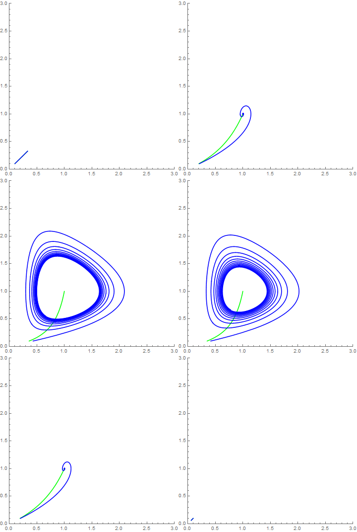
时滞/延迟微分方程(delay-differential equation)
问题
原来微分方程里面还有一类比较特殊复杂的。delay differential equation(维基).
翻了几篇相关的硕士和博士论文,感觉用处不大。不过,用软件做出来效果比较漂亮。
与之相关的, 分支或分叉(bifurcation)是一个似乎在包括迭代的动力系统里面都普遍的一个概念。
Wolfram关于这个概念的文档
延迟微分方程是一种微分方程,其在当前时间的时间导数取决于它在以往时间的解,还可能取决于它在以往时间的导数:
目前,在
NDSolve中延迟微分方程的实现只支持常量延迟.虽然延迟微分方程看起来很像常微分方程,它们的理论更加复杂,并且与常微分方程有一些令人吃惊的不同之处
同样是数值计算,更愿意用mathematica而不是可能更强的matlab, 主要是演示效果吧。
Mathworks关于这个概念的文档
Matlab中Delay Differential Equations求解用到的函数
论文一篇:用Matlab解DDE(2001):
| No. | Delay differential equation initial value problem solvers | Functions |
|---|---|---|
| 1 | dde23 |
Solve delay differential equations (DDEs) with constant delays |
| 2 | ddesd |
Solve delay differential equations (DDEs) with general delays |
| 3 | ddensd |
Solve delay differential equations (DDEs) of neutral type |
| 4 | ddeget |
Extract properties from delay differential equations options structure |
| 5 | ddeset |
Create or alter delay differential equations options structure |
| 6 | deval |
Evaluate solution of differential equation problem |
一些演示
其它软件很少有这种特色的论坛:
First, I have a few general comments. The simplest bifurcation diagrams for differential equations involve a single parameter in a single equation and there are several illustrations of these on the Wolfram Demonstrations site. More generally, of course, a bifurcation occurs when we see a qualitative change in the behavior of a system as some parameter changes. For a system of equations, we could use the eigensystem of the linearization of the system in the neighborhood of an equilibrium to identify bifuractions. You, however, appear to have four differential-algebraic equations with 16 parameters. Also, a number of these (K, I, E, N) are actually reserved symbols; I’d avoid that.
I don’t think I’m going to wade into this system that I know nothing about but I can present some ideas to study this kind of thing in the context of an example that I understand, namely the Selkov model presented on the Demonstrations site:
That demonstration shows you how to study the bifurcation using NDSolve. It might make sense to study it using the groovy new ParametricNDSolve. First, the system is the following:
pf = ParametricNDSolveValue[{
 x'[t] == -x[t] + a*y[t] + x[t]^2 y[t],
 y'[t] == b - a*y[t] - x[t]^2*y[t],
 x[0] == 0, y[0] == 2},
 {x, y}, {t, 0, 100}, {a, b}];
We can investigate the behavior with respect to the parameters as follows. If you hold a=0.1 and let be range, a two Hopf bifurcations (changes from fixed point to cycle and back) should be evident
Manipulate[
 Block[{$PerformanceGoal = "Quality"},
 Show[{
 ContourPlot[-x + a*y + x^2 y == 0, {x, 0, 3}, {y, 0, 3},
 ContourStyle -> Dashed],
 ContourPlot[b - a*y - x^2*y == 0, {x, 0, 3}, {y, 0, 3},
 ContourStyle -> Dashed],
 StreamPlot[{-x + a*y + x^2 y, b - a*y - x^2*y},
 {x, 0, 3}, {y, 0, 3},
 StreamStyle -> Directive[Opacity[0.5]]],
 ParametricPlot[
 Evaluate[Through[pf[a, b][t]]],
 {t, 0, 100}, PlotRange -> {{0, 3}, {0, 3}},
 PlotStyle -> Directive[Thickness[0.007], Black]]}]],
 {{a, 0.1}, 0, 1}, {b, 0, 1}]
