机器学习实战第三章（决策树）

第二章介绍的k-近邻算法可以完成很多分类任务，但是最大缺点是无法给出数据的内在含义，决策树的主要优势就在于数据形式非常容易理解。

决策树：
优点：计算复杂度不高，输出结果易于理解，对中间值的缺失不敏感，可以处理不相关特征数据
缺点：可能会产生过度匹配问题
树用数据类型：数值型和标称型。

在构造决策树时，我们需要解决的第一个问题就是，当前数据集上哪个特征在划分数据分类时起决定性作用。为了找到决定性的特征，划分出最好的结果，我们必须评估每个特征。我们假设已经根据一定的方法选取了待划分的特征，则原始数据集将根据这个特征被划分为几个数据子集。这数据子集会分布在决策点（关键特征）的所有分支上。如果某个分支下的数据属于同一类型，则无需进一步对数据集进行分割。如果数据子集内的数据不属于同一类型，则需要递归地重复划分数据子集的过程，直到每个数据子集内的数据类型相同。
创建分支的过程用伪代码表示如下：
- 检测数据集中的每个子项是否属于同一类型：
　　如果是，则返回类型标签
　　否则：
　　　　寻找划分数据集的最好特征
　　　　划分数据集
　　　　创建分支节点
　　　　对划分的每个数据子集：
　　　　　　递归调用本算法并添加返回结果到分支节点中
　　　　返回分支节点

决策树的一般流程：

1. 收集数据：可以使用任何方法。
2. 准备数据：树构造算法只适用于标称数据，因此数值型数据必须离散化。
3. 分析数据：可以使用任何方法，构造树完成之后，我们应该检查图形是否符合预期。
4. 训练算法：构造树的数据结构。
5. 测试算法：使用经验树计算错误率。
6. 使用算法：此步骤可以适用于任何监督学习算法，而使用决策树可以更好地理解数据的内在含义。

一些决策树算法使用二分法划分数据，本书并不采用这种方法。如果依据某个属性划分数据将会产生4个可能的值，我们将把数据划分成四块，并创建四个不同的分支。

本书将使用ID3算法划分数据集，该算法处理如何划分数据集，何时停止划分数据集（进一步的信息可以参见http://en.wikipedia.org/wiki/ID3_algorithm）。每次划分数据集我们只选取一个特征属性，那么应该选择哪个特征作为划分的参考属性呢？

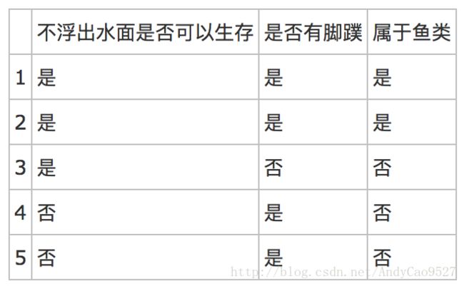
表1的数据包含5个海洋动物，特征包括：不浮出水面是否可以生存，以及是否有脚噗。我们可以将这些动物分成两类：鱼类和非鱼类。现在我们想要决定依据第一个特征还是第二个特征划分数据。在回答这个问题之前，我们必须采用量化的方法判断如何划分数据

信息增益

划分数据集的大原则是：将无序的数据变得更加有序。我们可以使用多种方法划分数据集，但是每种方法都有各自的优缺点。组织杂乱无章数据的一种方法就是使用信息论度量信息，信息论是量化处理信息的分支科学。我们可以在划分数据之前或之后使用信息论量化度量信息的内容。

在划分数据集之前之后信息发生的变化成为信息增益，我们可以计算每个特征划分数据集获得的信息增益，获得信息增益最高的特征就是最好的选择。

集合信息的度量方式成为香农熵或者简称为熵。

熵定义为信息的期望值。我们先确定信息的定义：

如果待分类的事务可能划分在多个分类之中，则符号xi定义为：

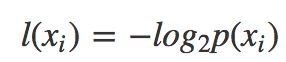
其中p(xi)是选择该分类的概率。

为了计算熵，我们需要计算所有类型所有可能值包含的信息的期望值，通过下面的公式得到：

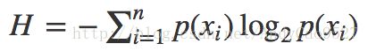
其中n是分类的数目。

创建简单的鱼鉴定数据集

# -*- coding: UTF-8 -*- 

from math import log

def createDataSet():  #创建数据集
    dataSet = [
        [1,1,'yes'],
        [1,1,'yes'],
        [1,0,'no'],
        [0,1,'no'],
        [0,1,'no']
    ]

    labels = ['no surfacing', 'flippers']
    return dataSet, labels

myDat, labels = createDataSet() print myDat, labels

output:
[[1, 1, ‘yes’], [1, 1, ‘yes’], [1, 0, ‘no’], [0, 1, ‘no’], [0, 1, ‘no’]]
[‘no surfacing’, ‘flippers’]

程序清单3-1 计算给定数据集的信息熵

def calcShannonEnt(dataSet): #计算给定数据集的香农熵
    numEntries = len(dataSet) #计算数据集中的实例总数
    labelCounts = {}
    for featVec in dataSet:
        currentLabel = featVec[-1]
        #print currentLabel
        if currentLabel not in labelCounts.keys():
            labelCounts[currentLabel] = 0
        labelCounts[currentLabel] += 1

    shannonEnt = 0.0
    for key in labelCounts:
        prob = float(labelCounts[key])/numEntries
        shannonEnt -= prob * log(prob,2)
    return shannonEnt

代码说明：

• 首先，计算数据集中实例的总数。我们可以在需要时再计算这个值，但是由于代码中多次用到这个值，为了提高代码效率，我们显式地声明一个变量保存实例总数。
• 然后，创建一个数据字典，它的键值是最后一列的数值。如果当前键值不存在，则扩展字典并将当前键值加入字典。每个键值都记录了当前类别出现的粗疏。
• 最后，使用所有类标签的发生频率计算类别出现的概率。我们将用这个概率计算香农熵，统计所有类标签发生的次数。

熵越高，则混合的数据越多，我们可以在数据集中添加更多的分类，观察熵是如何变化的

print calcShannonEnt(myDat)

output：
0.970950594455

myDat[0][-1]='caoxin'
print calcShannonEnt(myDat)

output：
1.37095059445

得到熵之后，我们就可以按照最大信息增益的方法划分数据集。
另一个度量集合无序程度的方法是基尼不纯度（Gini impurity），简单地说就是从一个数据集中随机选取子项，度量其被错误分类到其他分组里的概率。

划分数据集 ##

上节学习了如何度量数据集的无序程度，分类算法除了需要测量信息熵，还需要划分数据集，度量花费数据集的熵，以便判断当前是否正确划分了数据集。我们将对每个特征划分数据集的结果计算一次信息熵，然后判断按照哪个特征划分数据集是最好的划分方法。

程序清单3-2 按照给定特征划分数据集

def splitDataSet(dataSet, axis, value):#三个输入参数：带划分的数据集、划分数据集的特征、需要返回的特征的值
    retDataSet = []
    for featVec in dataSet:
        #print featVec
        #print axis,value
        if featVec[axis] == value:
            reducedFeatVec = featVec[:axis]
            reducedFeatVec.extend(featVec[axis+1:])
            retDataSet.append(reducedFeatVec)
    return retDataSet

extend 和 append的却别

a=[1,2,3]
b=[4,5,6]
a.extend(b)
print a

output:
[1, 2, 3, 4, 5, 6]

a=[1,2,3]
b=[4,5,6]
a.append(b)
print a

output:
[1, 2, 3, [4, 5, 6]]

print myDat
print splitDataSet(myDat,1,1)    

output:
[[1, 1, ‘yes’], [1, 1, ‘yes’], [1, 0, ‘no’], [0, 1, ‘no’], [0, 1, ‘no’]]
[[1, ‘yes’], [1, ‘yes’], [0, ‘no’], [0, ‘no’]]

接下来遍历整个数据集，循环计算香农熵和splitDataSet()函数，找到最好的特征划分方式。熵计算将会告诉我们如何划分数据集释最好的数据组织方式。
程序清单3-3 选择最好的数据集划分方式

def chooseBestFeatureToSplit(dataSet):
    numFeatures = len(dataSet[0]) - 1
    baseEntropy = calcShannonEnt(dataSet)
    bestInfoGain = 0.0
    bestFeature = -1
    for i in range(numFeatures):1 
        featList = [example[i] for example in dataSet]
        uniqueVals = set(featList)
        newEntropy = 0.0
        for value in uniqueVals: 
            subDataSet = splitDataSet(dataSet, i, value) 
            prob = len(subDataSet)/float(len(dataSet))
            newEntropy += prob * calcShannonEnt(subDataSet)
        infoGain = baseEntropy - newEntropy
        if (infoGain > bestInfoGain):
            bestInfoGain = infoGain
            bestFeature = i
    return bestFeature

• 本函数使用变量bestInfoGain和bestFeature记录最好的信息增益和对应的特征；
• numFeatures记录特征维数，依次遍历各个特征，计算该特征值的集合（uniqueVals）；
• 遍历该特征计算使用该特征划分的熵（newEntropy），据此计算新的信息增益（infoGain）；
• 比较infoGain和bestInfoGain记录信息增益的最大值和对应特征；
• 最终返回最大的信息增益对应特征的索引。

print chooseBestFeatureToSplit(myDat)

output:
0
函数选取了第一个特征用于划分。

递归决策树构建

构造决策树所需的子功能模块已经介绍完毕，构建决策树的算法流程如下：

1. 得到原始数据集
2. 基于最好的属性值划分数据集，由于特征值可能多于两个，因此可能存在大于两个分支的数据集划分。
3. 第一次划分之后，数据将被向下传递到树分支的下一个节点，在这个节点上，我们可以再次划分数据。我们可以采用递归的原则处理数据集。

4. 递归结束的条件是，程序遍历完所有划分数据集的属性，或者每个分支下的所有实例都具有相同的分类。

   添加如下代码：

def majorityCnt(classList): #返回出现次数最多的分类名称
    classCount={}
    for vote in classList:
        if vote not in classCount.keys():
            classCount[vote] = 0
        classCount[vote] += 1
    sortedClassCount = sorted(classCount.iteritems(), key=operator.itemgetter(1), reverse=True)
    return sortedClassCount[0][0] 

程序清单3-4 创建树的函数代码

def createTree(dataSet,labels):
    classList = [example[-1] for example in dataSet] #包含了数据集的所有类标签
    #递归函数第一个停止的条件是所有的类标签完全相同，则返回该类标签
    if classList.count(classList[0]) == len(classList): 
        return classList[0]
    #递归函数第二个停止的条件是使用完了所有的特征，仍然不能将数据集划分成仅包含唯一类别的分组
    if len(dataSet[0]) == 1:
        #majorityCnt函数统计classList列表中每个类型标签出现频率，返回出现次数最多的分类名称。
        return majorityCnt(classList)
    bestFeat = chooseBestFeatureToSplit(dataSet) #当前数据集选取的最好特征存储在变量bestFeat中
    bestFeatLabel = labels[bestFeat]
    myTree = {bestFeatLabel:{}} #将决策树存在字典中
    del(labels[bestFeat]) #labels删除当前使用完的特征值的label
    featValues = [example[bestFeat] for example in dataSet]
    uniqueVals = set(featValues)
    #递归输出决策树
    for value in uniqueVals:
        subLabels = labels[:]
        myTree[bestFeatLabel][value] = createTree(splitDataSet(dataSet,bestFeat,value),subLabels)
    return myTree

myTree = createTree(myDat,labels) print myTree

output：
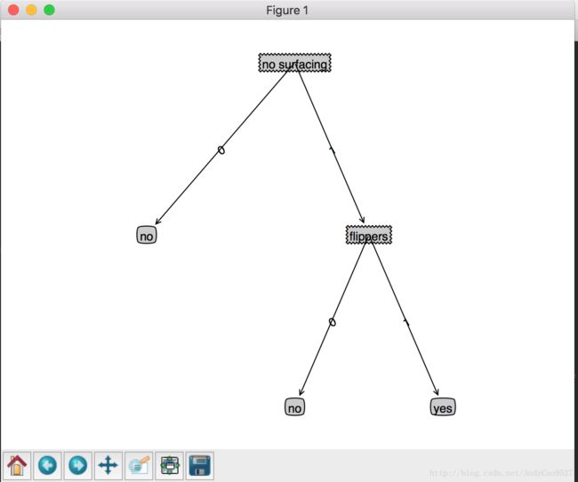
{‘no surfacing’: {0: ‘no’, 1: {‘flippers’: {0: ‘no’, 1: ‘yes’}}}}

从数据集构造决策树算法工作原理：
得到原始数据集，然后基于最好的属性值划分数据集，由于特征值可能多于两个，因此可能存在大雨两个分支的数据集划分，第一次划分之后，数据将被向下传递到树分支的下一个节点，在这个节点上，我们可以再次划分数据。因此可以采用递归的原则处理数据集。

递归结束的条件是：
程序遍历完所有划分数据集的属性
或者每个分支下的所有实例都具有相同的分类

如果所有实例具有相同的分类，则得到的一个叶子节点或者终止块。任何到达叶子节点的数据必然属于叶子节点的分类

在python中使用Matplotlib注解绘制树形图

# -*- coding: UTF-8 -*- 
import matplotlib.pyplot as plt


decisionNode = dict(boxstyle = 'sawtooth', fc = '0.8')
leafNode = dict(boxstyle = 'round4', fc = '0.8')
arrow_args = dict(arrowstyle = '<-')


def plotNode(nodeTxt, centerPt, parentPt, nodeType):
    createPlot.ax1.annotate(nodeTxt, xy = parentPt, xycoords = 'axes fraction', xytext = centerPt, textcoords = 'axes fraction', va = 'center', ha = 'center', bbox = nodeType, arrowprops = arrow_args)

''' def createPlot(): fig = plt.figure(1, facecolor = 'white') fig.clf() createPlot.ax1 = plt.subplot(111, frameon = False) plotNode('a decision node', (0.5, 0.1), (0.1, 0.5), decisionNode) plotNode('a leaf node', (0.8, 0.1), (0.3, 0.8), leafNode) plt.show() '''    
#createPlot()

def createPlot(inTree):
    fig = plt.figure(1, facecolor='white')
    fig.clf()
    axprops = dict(xticks=[], yticks=[])
    createPlot.ax1 = plt.subplot(111, frameon=False, **axprops)    #no ticks
    #createPlot.ax1 = plt.subplot(111, frameon=False) #ticks for demo puropses 
    plotTree.totalW = float(getNumLeafs(inTree))
    plotTree.totalD = float(getTreeDepth(inTree))
    plotTree.xOff = -0.5/plotTree.totalW; plotTree.yOff = 1.0;
    plotTree(inTree, (0.5,1.0), '')
    plt.show()

def getNumLeafs(myTree):
    numLeafs = 0
    firstStr = myTree.keys()[0]
    #print firstStr
    secondDict = myTree[firstStr]
    #print secondDict
    for key in secondDict.keys():
        #print 'key = ', key
        #print secondDict[key]
        if type(secondDict[key]).__name__=='dict':
            numLeafs += getNumLeafs(secondDict[key])
            #print 'numLeafs0=', numLeafs
        else:   
            numLeafs +=1
            #print 'numLeafs1=', numLeafs

    return numLeafs

def getTreeDepth(myTree):
    maxDepth = 0
    firstStr = myTree.keys()[0]
    #print firstStr
    secondDict = myTree[firstStr]
    #print secondDict
    for key in secondDict.keys():
        #print key
        #print secondDict[key]
        if type(secondDict[key]).__name__=='dict':

            thisDepth = 1 + getTreeDepth(secondDict[key])
            #print 'thisDepth0=', thisDepth
        else:   thisDepth = 1
        if thisDepth > maxDepth: maxDepth = thisDepth
    return maxDepth

testTree = {'no surfacing': {0: 'no', 1: {'flippers': {0: 'no', 1: 'yes'}}}}

#print getNumLeafs(testTree)
#print getTreeDepth(testTree)

def plotTree(myTree, parentPt, nodeTxt):#if the first key tells you what feat was split on
    numLeafs = getNumLeafs(myTree)  #this determines the x width of this tree
    depth = getTreeDepth(myTree)
    firstStr = myTree.keys()[0]     #the text label for this node should be this
    cntrPt = (plotTree.xOff + (1.0 + float(numLeafs))/2.0/plotTree.totalW, plotTree.yOff)
    plotMidText(cntrPt, parentPt, nodeTxt)
    plotNode(firstStr, cntrPt, parentPt, decisionNode)
    secondDict = myTree[firstStr]
    plotTree.yOff = plotTree.yOff - 1.0/plotTree.totalD
    for key in secondDict.keys():
        if type(secondDict[key]).__name__=='dict':#test to see if the nodes are dictonaires, if not they are leaf nodes 
            plotTree(secondDict[key],cntrPt,str(key))        #recursion
        else:   #it's a leaf node print the leaf node
            plotTree.xOff = plotTree.xOff + 1.0/plotTree.totalW
            plotNode(secondDict[key], (plotTree.xOff, plotTree.yOff), cntrPt, leafNode)
            plotMidText((plotTree.xOff, plotTree.yOff), cntrPt, str(key))
    plotTree.yOff = plotTree.yOff + 1.0/plotTree.totalD
#if you do get a dictonary you know it's a tree, and the first element will be another dict

def plotMidText(cntrPt, parentPt, txtString):
    xMid = (parentPt[0]-cntrPt[0])/2.0 + cntrPt[0]
    yMid = (parentPt[1]-cntrPt[1])/2.0 + cntrPt[1]
    createPlot.ax1.text(xMid, yMid, txtString, va="center", ha="center", rotation=30)


createPlot(testTree)

output: