浅谈SVD分解和CUR分解

1.Power iteration

In mathematics, the power iteration (also known as power method) is an eigenvalue algorithm: given a matrix A , the algorithm will produce a number λ , which is the greatest (in absolute value) eigenvalue of A , and a nonzero vector v , the corresponding eigenvector of λ , such that Av=λv . The algorithm is also known as the Von Mises iteration.

The power iteration is a very simple algorithm, but it may converge slowly. It does not compute a matrix decomposition, and hence it can be used when {\displaystyle A} A is a very large sparse matrix.

When M is a stochastic matrix(随机矩阵), the limiting vector is the principal eigenvector (主特征向量, the eigenvector with the largest eigenvalue), and its corresponding eigenvalue is 1. This method for finding the principal eigenvector, called power iteration, works quite generally, although if the principal eigenvalue (eigenvalue associated with the principal eigenvector) is not 1, then as i grows, the ratio of Mi+1v to Miv approaches the principal eigenvalue while M iv approaches a vector (probably not a unit vector) with the same direction as the principal eigenvector.

1.2Power iteration算法

1.3实例

M=[3226],λ1=7,v1=[0.4470.894],λ2=2,v2=[0.894−0.447]

M=[3 2; 2 6];
x0=[1 1]';
err=1;
%对M采用power iteration
while (err>0.001)
    x1=M*x0/norm(M*x0);
    err=norm([x1-x0])
    x0=x1;
end
x1    %主特征向量
lamda1=x1'*M*x1    %主特征值

M1=M-lamda1*x1*x1'
%对M1采用power iteration 
x0=[1 1]';
err=1;
while (err>0.001)
    x2=M1*x0/norm(M1*x0);
    err=norm([x2-x0])
    x0=x2;
end
x2%第二特征向量
lamda2=x2'*M1*x2%第二特征值

容易知道采用迭代法球出来的特征对与定义法求出来的特征对非常接近。

2.Principal-Component Analysis

Principal-component analysis, or PCA, is a technique for taking a dataset consisting of a set of tuples representing points in a high-dimensional space and finding the directions along which the tuples line up best. The idea is to treat the set of tuples as a matrix M and find the eigenvectors for MMT or MTM .The matrix of these eigenvectors can be thought of as a rigid rotation in a high dimensional space. When you apply this transformation to the original data, the axis corresponding to the principal eigenvector is the one along which the points are most “spread out,” More precisely, this axis is the one along which the variance of the data is maximized. Put another way, the points can best be viewed as lying along this axis, with small deviations from this axis. Likewise,the axis corresponding to the second eigenvector (the eigenvector corresponding to the second-largest eigenvalue) is the axis along which the variance of distances from the first axis is greatest, and so on.

We can view PCA as a data-mining technique. The high-dimensional data can be replaced by its projection onto the most important axes. These axes are the onescorresponding to the largest eigenvalues. Thus, the original data is approximated by data with many fewer dimensions, which summarizes well the original data.

主成分分析（Principal Component Analysis，PCA）， 是一种统计方法。通过正交变换将一组可能存在相关性的变量转换为一组线性不相关的变量，转换后的这组变量叫主成分。主成分分析首先是由K.皮尔森（Karl Pearson）对非随机变量引入的，尔后H.霍特林将此方法推广到随机向量的情形。信息的大小通常用离差平方和或方差来衡量。

3. MMT 和 MTM 的共同特征值

对于 Mn×m 矩阵，矩阵 MMT 的特征值是矩阵 MTM 的特征值加上 n−m 个0，如果 n>m .反之也是成立，如果 n<m ，则矩阵 MTM 的特征值是矩阵 MMT 的特征值加上 n−m 个0

证明如下：
对于矩阵 Mn∗m ，我们假设 n>m ，假设 e 是 MTM 的一个特征向量， λ 是其对应的特征值，则有：

MTMe=λe⇒MMTMe=λMe⇒MMT(Me)=λ(Me)

此处，只要 Me 不是零向量，它则是 MMT 的特征向量，而 λ 这是 MTM 和 MMT 的共同特征值。

反过来也成立，我们假设 e 是 MMT 的一个特征向量， λ 是其对应的特征值，则有：

MMTe=λe⇒MTMMTe=λMTe⇒MTM(MTe)=λ(MTe)

此处，只要 MTe 不是零向量，它则是 MTM 的特征向量，而 λ 这是 MTM 和 MMT 的共同特征值。
当 MTe=0 时，会有 MMTe=0 ,而特征向量 e 是非零向量，则有 MMTe=0=λe ，由此推出 λ=0 .

至此，我们已经证明矩阵 MMT 的特征值是矩阵 MTM 的特征值加上 n−m 个0，如果 n>m .反之也是成立，如果 n<m ，则矩阵 MTM 的特征值是矩阵 MMT 的特征值加上 n−m 个0。

4.Singular-Value Decomposition（SVD）

We now take up a second form of matrix analysis that leads to a low-dimensional representation of a high-dimensional matrix. This approach, called singularvalue decomposition (SVD), allows an exact representation of any matrix, and also makes it easy to eliminate the less important parts of that representation to produce an approximate representation with any desired number of dimensions. Of course the fewer the dimensions we choose, the less accurate will be the approximation.

4.1SVD的定义

4.2SVD计算原理

4.2.1计算 V 矩阵

对于原始数据矩阵A,

A=UΣVT

由定义可知 Σ 为对角矩阵，即 Σ=ΣT ,则有

AT=(UΣVT)T=(VT)TΣTUT=VΣTUT=VΣUT

因此：

ATA=VΣUTUΣVT

由定义可知， U 矩阵为正交矩阵，即 UTU=I , I 为单位矩阵，上式等价于

ATA=VΣΣVT=VΣ2VT

上式两边同时左乘 V ,可得

ATAV=VΣ2VTV

而由定义可知矩阵 V 是正交矩阵，即 VTV=I ,I是单位矩阵，所以上式等价于：

ATAV=VΣ2

因为矩阵 Σ 是对角矩阵，因此矩阵 Σ2 也是对角矩阵，其对角元素是矩阵 Σ 对应的对角元素的平方。上式表明矩阵 Σ2 的对角元素是矩阵 ATA 的特征值，其对应的特征向量是矩阵 V 中的各个列向量。

4.2.2计算 U 矩阵

U 矩阵的计算方法与 V 矩阵的计算方法类似。

AAT=UΣVT(UΣVT)T=UΣVTVΣUT=UΣΣUT=UΣ2UT

上式两边同时左乘矩阵 U ,可得

AATU=UΣ2UTU=UΣ2

上式表明矩阵 Σ2 的对角元素是矩阵 AAT 的特征值，其对应的特征向量是矩阵 U 中的各个列向量。

A small detail needs to be explained concerning U and V . Each of these matrices have r columns, while ATA is an n×n matrix and AAT is an m×m matrix. Both n and m are at least as large as r . Thus, AAT and ATA should have an additional n−r and m−r eigenpairs, respectively, and these pairs donot show up in U , V , and Σ . Since the rank of A is r , all other eigenvalueswill be 0, and these are not useful.

4.3SVD的应用

Instance#1
there are two “concepts” underlying the movies: science-fiction and romance. All the boys rate only science-fiction, and all the girls rate only romance.

SVD分解如下：

The key to understanding what SVD offers is in viewing the r columns of U , Σ , and V as representing concepts that are hidden in the original matrix M . In Example 11.8, these concepts are clear; one is “science fiction” and the other is “romance.” Let us think of the rows of M as people and the columns of M as movies. Then matrix U connects people to concepts. For example, the person Joe, who corresponds to row 1 of M in Fig. 11.6, likes only the concept science fiction. The value 0.14 in the first row and first column of U is smaller than some of the other entries in that column, because while Joe watches only science fiction, he doesn’t rate those movies highly. The second column of the first row of U is 0, because Joe doesn’t rate romance movies at all.

The matrix V relates movies to concepts. The 0.58 in each of the first three columns of the first row of VT indicates that the first three movies – Matrix, Alien, and Star Wars – each are of the science-fiction genre, while the 0’s in the last two columns of the first row say that these movies do not partake of the concept romance at all. Likewise, the second row of VT tells us that the movies Casablanca and Titanic are exclusively romances.

Finally, the matrix Σ gives the strength of each of the concepts. In our example, the strength of the science-fiction concept is 12.4, while the strength of the romance concept is 9.5. Intuitively, the science-fiction concept is stronger because the data provides more movies of that genre and more people who like them.

SVD-Interpretation #2
Dimensionality Reduction Using SVD

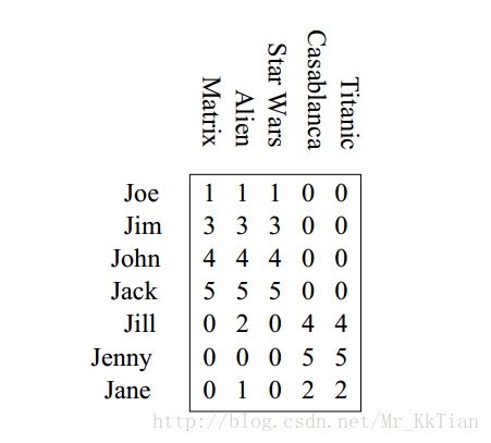
进行SVD分解如下：

Suppose we want to represent a very large matrix M by its SVD components U , Σ , and V , but these matrices are also too large to store conveniently. The best way to reduce the dimensionality of the three matrices is to set the smallest of the singular values to zero. If we set the s smallest singular values to 0, then we can also eliminate the corresponding s rows of U and V .

Suppose we want to reduce the number of dimensions to two. Then we set the smallest of the singular values, which is 1.3, to zero. The effect on the expression in Fig. 11.9 is that the third column of U and the third row of VT are multiplied only by 0’s when we perform the multiplication, so this row and this column may as well not be there. That is, the approximation to M' obtained by using only the two largest singular values is that shown in Fig. 11.10.

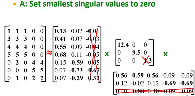
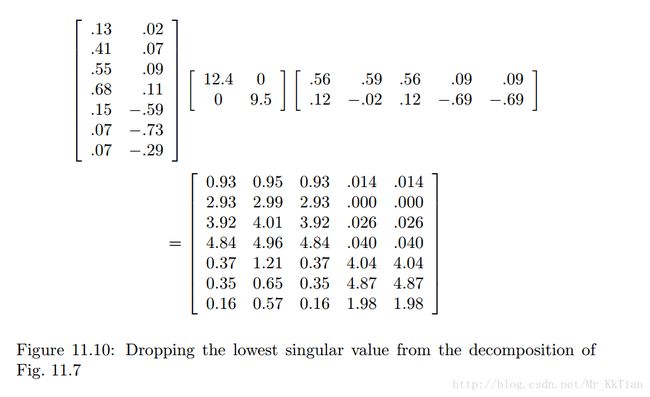
The resulting matrix is quite close to the matrix M' of Fig. 11.8. Ideally, the entire difference is the result of making the last singular value be 0. However, in this simple example, much of the difference is due to rounding error caused by the fact that the decomposition of M' was only correct to two significant digits.

关于为什么选择较小的特征值设置为0，选择哪些个特征值并设置为0可以得到很好的降维效果，以及为什么这样处理的SVD非常有效可以参看《Mining of massive datasets》

5.PCA与SVD比较

6.CUR Decomposition(CUR分解)

In large-data applications, it is normal for the matrix M being decomposed to be very sparse; that is, most entries are 0. For example, a matrix representing many documents (as rows) and the words they contain (as columns) will be sparse, because most words are not present in most documents. Similarly, a matrix of customers and products will be sparse because most people do not buy most products.

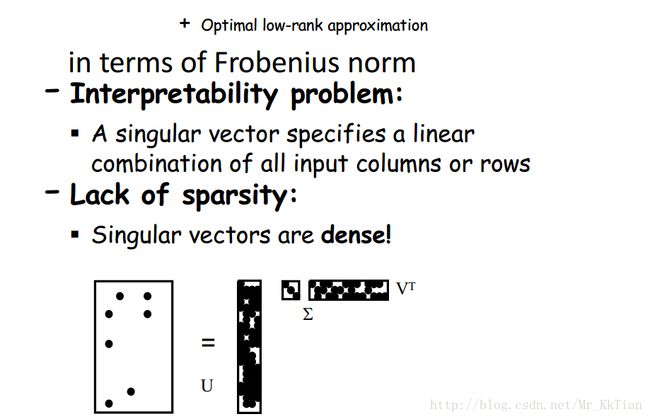
We cannot deal with dense matrices that have millions or billions of rows and/or columns. However, with SVD, even if M is sparse, U and V will be dense. Σ , being diagonal, will be sparse, but Σ is usually much smaller than U and V ,so its sparseness does not help.

SVD分解的劣势如下：

It is common for the matrix M that we wish to decompose to be very sparse.
But U and V from a UV or SVD decomposition will not be sparse even so.
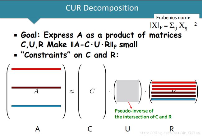
CUR decomposition solves this problem by using only (randomly chosen) rows and columns of M.

6.1CUR分解的定义

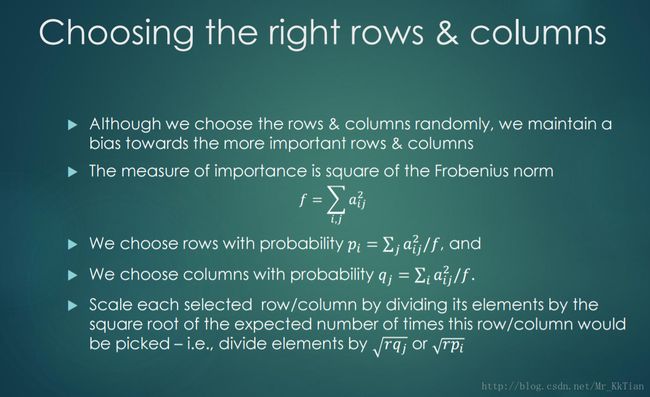
6.1.1矩阵 C R 的构建方法

随机选择具体算法伪代码如下:

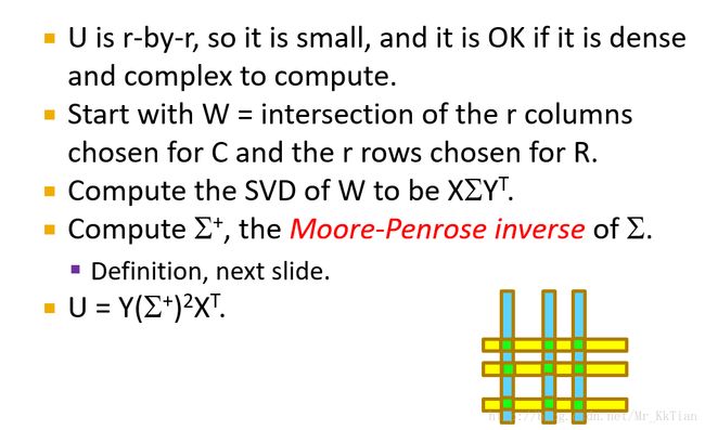
6.1.2 U 矩阵的构建方法如下:

Moore-Penrose Inverse的定义如下：

CUR分解可以看成如下的优化问题：

6.2 SVD vs CUR

Ref:
https://en.wikipedia.org/wiki/CUR_matrix_approximation
http://web.stanford.edu/class/cs246/handouts.html