下采样及过采样·交叉验证及混淆矩阵【知识整理】

综述

学生党整理一些关于数据分析的知识：主要整理了下采样和过采样这两个采样方式。采用召回率（Recall）作为评估标准，此外还采用了交叉验证划分样本引人正则惩罚项对切分的训练数据循环验证、用混淆矩阵展示最优结果。进一步探究两种采样方式的优劣。

代码模块

调用库

import pandas as pd
import numpy as np
import matplotlib.pyplot as plt

数据样例

拿到数据后我们需要明确我们的目标是什么，要采用那些方法实现。
我们现在以一组病人数据为例，先读入数据：

data = pd.read_csv('creditcard.csv')
print(data.head())

结果如下：

   Time        V1        V2        V3  ...       V27       V28  Amount  Class
0   0.0 -1.359807 -0.072781  2.536347  ...  0.133558 -0.021053  149.62      0
1   0.0  1.191857  0.266151  0.166480  ... -0.008983  0.014724    2.69      0
2   1.0 -1.358354 -1.340163  1.773209  ... -0.055353 -0.059752  378.66      0
3   1.0 -0.966272 -0.185226  1.792993  ...  0.062723  0.061458  123.50      0
4   2.0 -1.158233  0.877737  1.548718  ...  0.219422  0.215153   69.99      0

[5 rows x 31 columns]

每个样本都有31个特征，现在我们要分析病人是不是癌症病人这个特征和其他30个特征的关系。首先病人是否患癌症是个二分类问题。
绘制条形图观察Class特征：

count_class = pd.value_counts(data['Class'],sort=True).sort_index()
count_class.plot(kind = 'bar',color = 'darkblue')
plt.xlabel('Class')
plt.ylabel('Freqquency')
plt.show()

结果如下：

明显看出大部分病人未患癌症，极小部分的病人才患有癌症。显然我们的样本是不平衡的，所以我们采用下采样或过采样的方法，让患癌和未患癌的样本数量平衡。

下采样

目前两个样本的数量不同，为了让样本一样少，从 0 号样本中选取和 1 号样本数量一同的样本量
首先，让每个特征的重要性相同，对数据做归一化或者标准化处理，消除数字上的差异：

from sklearn.preprocessing import StandardScaler
# 数据标准化
data['normAmount'] = StandardScaler().fit_transform(data['Amount'].values.reshape(-1,1))#-1为自动识别，在元素个数固定时一个量可以自己算
data = data.drop(['Time','Amount'],axis=1) #去除不需要的特征
print(data.head())

下采样处理：

X = data.ix[:,data.columns != 'Class']
y = data.ix[:,data.columns == 'Class']

# 让0和1 一样少
number_one = len(data[data['Class'] == 1])
fruad_indices = np.array(data[data.Class == 1].index)

number_zero = len(data[data['Class'] == 0].index)

random_normal_indices = np.random.choice(number_zero,number_one,replace=False)
random_normal_indices = np.array(random_normal_indices)

under_sample_indices = np.concatenate([fruad_indices,random_normal_indices])
under_sample_data = data.iloc[under_sample_indices,:]

X_undersample = under_sample_data.ix[:,under_sample_data.columns != 'Class']
y_undersample = under_sample_data.ix[:,under_sample_data.columns == 'Class']

#显示下采样后的数据
print("Perentage of normal transactions:",len(under_sample_data[under_sample_data.Class == 0])/len(under_sample_data))
print("Perentage of fraud transactions:",len(under_sample_data[under_sample_data.Class == 1])/len(under_sample_data))
print("Total number of transactions in resampled data:",len(under_sample_data))

结果显示：

Perentage of normal transactions: 0.5
Perentage of fraud transactions: 0.5
Total number of transactions in resampled data: 984

划分训练集和测试集

数据切分：（旧版库为sklearn.cross_validation）：

• 原始数据

from sklearn.model_selection import train_test_split
#原始数据
X_train, X_test, y_train, y_test = train_test_split(X,y,test_size=0.3,random_state= 0) #测试数据为30%
print('Number trainsactions train dataset:',len(X_train))
print('Number trainsactions test dataset:',len(X_test))
print('Number trainsactions dataset:',len(X_train)+len(X_test))

结果：

Number trainsactions train dataset: 199364
Number trainsactions test dataset: 85443
Number trainsactions dataset: 284807

• 样本数据

X_train_undersample, X_test_undersample, y_train_undersample, y_test_undersample = train_test_split(X_undersample,y_undersample,test_size=0.3,random_state= 0) #测试数据为30%
print('Number trainsactions train dataset:',len(X_train_undersample))
print('Number trainsactions test dataset:',len(X_test_undersample))
print('Number trainsactions dataset:',len(X_train_undersample)+len(X_test_undersample))

结果：

Number trainsactions train dataset: 688
Number trainsactions test dataset: 296
Number trainsactions dataset: 984

交叉验证

交叉验证：将train分成3份（A，B，C），这时我们训练A+B测试C，再训练A+C测试B及B+C训练验证A。这样的过程叫交叉验证，3次评估的均值表示模型效果。
再进行交叉验证之前我要先解决评估标准的问题：二分类问题中只采用精度作为评估标准是不可靠的，再对小概率事件做预测时，例如1000个病人中有10个是患癌症的。当你的模型预测出来全部为正时，你的精度得到99%，显然是不正确的。所以我们还要采用Recall召回率（查全率），即预测出癌症人数的准确度（预测人数/实际人数）作为评价标准。具体的检验方式为：

	相关(Relevant),正类	无关(NonRelevant),负类
被检索到 \newline (Retrieved)	true postives(TP)	false positives(FP)
未被检索到 \newline (NonRetrieved)	false negatives(FN)	true negatives(TN)

对于本文的数据案例来看，我们支持原假设未患癌症为 positives 那么正确判断的为TP和TN，错误判断的为FP和FN。
计算公式为：$$Recall=TP/(TP+FN)$$

此外，定义了 0.01,0.1,1,10,100 五个正则惩罚力度

• 交叉验证模块：

from sklearn.linear_model import LogisticRegression
from sklearn.model_selection import cross_val_score,KFold   #切分，交叉验证得分
from sklearn.metrics import confusion_matrix,recall_score,classification_report #混淆矩阵

def printing_Kflod_scores(x_train_data,y_train_data):
    fold = KFold(5,shuffle=False)#切分5部分

    c_param_range = [0.01,0.1,1,10,100] #正则化惩罚项（惩罚力度）

    results_table = pd.DataFrame(index= range(len(c_param_range)),columns = ['C_parametet','Mean recall score'])
    results_table['C_parameter'] = c_param_range
    print(results_table)
    '''
	      C_parametet Mean recall score  C_parameter
	0         NaN               NaN         0.01
	1         NaN               NaN         0.10
	2         NaN               NaN         1.00
	3         NaN               NaN        10.00
	4         NaN               NaN       100.00
    '''

    j = 0
    best = []
    for c_param in c_param_range:
        print('-----------------------------------')
        print('C parameter:',c_param)
        print('-----------------------------------')
        print('')

        recall_accs = []
        # 使用5中惩罚，观察那种惩罚的效果好，对5个部分循环验证
        for iteration, indices in enumerate(fold.split(x_train_data)):

            lr = LogisticRegression(C = c_param, penalty= 'l1',solver='liblinear')#逻辑回归，（惩罚力度，惩罚方法【l1（1/2w^2），l2（|w|）】）
            # 训练数据
            lr.fit(x_train_data.iloc[indices[0],:],y_train_data.iloc[indices[0],:].values.ravel())
            #预测
            y_pred_undersample = lr.predict(x_train_data.iloc[indices[1],:].values)

            recall_acc = recall_score(y_train_data.iloc[indices[1],:].values,y_pred_undersample)
            recall_accs.append(recall_acc)
            print('Iteration',str(int(iteration)+1),':recall score = ',recall_acc)

        results_table.ix[j,'Mean recall score'] = np.mean(recall_accs)
        j += j
        print('')
        best_c_now = np.mean(recall_accs)
        print('Mean recall score ',best_c_now)
        best.append(best_c_now)
        print('')
    best_c = c_param_range[best.index(max(best))]
    print('The best c',best_c)
    return best_c

best_c = printing_Kflod_scores(X_train_undersample,y_train_undersample)

结果如下：

-----------------------------------
C parameter: 0.01
-----------------------------------

Iteration 1 :recall score =  0.9452054794520548
Iteration 2 :recall score =  0.9178082191780822
Iteration 3 :recall score =  1.0
Iteration 4 :recall score =  0.972972972972973
Iteration 5 :recall score =  0.9545454545454546

Mean recall score  0.9581064252297129

-----------------------------------
C parameter: 0.1
-----------------------------------

Iteration 1 :recall score =  0.8493150684931506
Iteration 2 :recall score =  0.863013698630137
Iteration 3 :recall score =  0.9661016949152542
Iteration 4 :recall score =  0.9324324324324325
Iteration 5 :recall score =  0.8939393939393939

Mean recall score  0.9009604576820737

-----------------------------------
C parameter: 1
-----------------------------------

Iteration 1 :recall score =  0.8767123287671232
Iteration 2 :recall score =  0.8904109589041096
Iteration 3 :recall score =  0.9830508474576272
Iteration 4 :recall score =  0.9459459459459459
Iteration 5 :recall score =  0.9090909090909091

Mean recall score  0.921042198033143

-----------------------------------
C parameter: 10
-----------------------------------

Iteration 1 :recall score =  0.8767123287671232
Iteration 2 :recall score =  0.8904109589041096
Iteration 3 :recall score =  0.9830508474576272
Iteration 4 :recall score =  0.9324324324324325
Iteration 5 :recall score =  0.9090909090909091

Mean recall score  0.9183394953304402

-----------------------------------
C parameter: 100
-----------------------------------

Iteration 1 :recall score =  0.8767123287671232
Iteration 2 :recall score =  0.8904109589041096
Iteration 3 :recall score =  0.9830508474576272
Iteration 4 :recall score =  0.9459459459459459
Iteration 5 :recall score =  0.9090909090909091

Mean recall score  0.921042198033143

The best c 0.01
Recall metric in the testing dataset:  0.9387755102040817

混淆矩阵

混淆矩阵：用图像表示Recall，精度正好等于正对角线合/总数量
混淆矩阵模块：

def plot_confusion_matrix(cm, classes,
                          title='Confusion matrix',
                          cmap=plt.cm.Blues):
    """
    This function prints and plots the confusion matrix.
    """
    plt.imshow(cm, interpolation='nearest', cmap=cmap)
    plt.title(title)
    plt.colorbar()
    tick_marks = np.arange(len(classes))
    plt.xticks(tick_marks, classes, rotation=0)
    plt.yticks(tick_marks, classes)

    thresh = cm.max() / 2.
    for i, j in itertools.product(range(cm.shape[0]), range(cm.shape[1])):
        plt.text(j, i, cm[i, j],
                 horizontalalignment="center",
                 color="white" if cm[i, j] > thresh else "black")

    plt.tight_layout()
    plt.ylabel('True label')
    plt.xlabel('Predicted label')

对测试集检验：

import itertools

def mixfig_down():
    lr = LogisticRegression(C=best_c, penalty='l1',solver='liblinear')
    lr.fit(X_train_undersample, y_train_undersample.values.ravel())
    y_pred_undersample = lr.predict(X_test_undersample.values)

    # Compute confusion matrix
    cnf_matrix = confusion_matrix(y_test_undersample, y_pred_undersample)
    np.set_printoptions(precision=2)

    print("Recall metric in the testing dataset: ", cnf_matrix[1, 1] / (cnf_matrix[1, 0] + cnf_matrix[1, 1]))

    # Plot non-normalized confusion matrix
    class_names = [0, 1]
    plt.figure()
    plot_confusion_matrix(cnf_matrix
                          , classes=class_names
                          , title='Confusion matrix')
    plt.show()

    #用下采样训练的模型验证原本的总样本
    #lr = LogisticRegression(C=best_c, penalty='l1',solver='liblinear')
    lr.fit(X_train_undersample, y_train_undersample.values.ravel())
    y_pred = lr.predict(X_test.values)
    # Compute confusion matrix
    cnf_matrix = confusion_matrix(y_test,y_pred)
    np.set_printoptions(precision=2)

    print("Recall metric in the testing dataset: ", cnf_matrix[1, 1] / (cnf_matrix[1, 0] + cnf_matrix[1, 1]))

    # Plot non-normalized confusion matrix
    class_names = [0, 1]
    plt.figure()
    plot_confusion_matrix(cnf_matrix
                          , classes=class_names
                          , title='Confusion matrix')
    plt.show()

mixfig_down()

结果：

Recall metric in the testing dataset:  0.9387755102040817

Recall metric in the testing dataset:  0.9251700680272109

虽然模型得出的Recall值不错，但是从混淆矩阵来看NP的数量过大了，对整体测试集的预测显然超出了合理范围。

阈值调整

为了解决模型结果不理想，可以考虑变更分界线的阈值（默认情况下为0.5）

def threshold():
    lr = LogisticRegression(C=0.01, penalty='l1',solver='liblinear')
    lr.fit(X_train_undersample, y_train_undersample.values.ravel())
    y_pred_undersample_proba = lr.predict_proba(X_test_undersample.values)

    thresholds = [0.1, 0.2, 0.3, 0.4, 0.5, 0.6, 0.7, 0.8, 0.9]

    plt.figure(figsize=(10, 10))

    j = 1
    for i in thresholds:
        y_test_predictions_high_recall = y_pred_undersample_proba[:, 1] > i

        plt.subplot(3, 3, j)
        j += 1

        # Compute confusion matrix
        cnf_matrix = confusion_matrix(y_test_undersample, y_test_predictions_high_recall)
        np.set_printoptions(precision=2)

        print("Recall metric in the testing dataset: ", cnf_matrix[1, 1] / (cnf_matrix[1, 0] + cnf_matrix[1, 1]))

        # Plot non-normalized confusion matrix
        class_names = [0, 1]
        plot_confusion_matrix(cnf_matrix
                              , classes=class_names
                              , title='Threshold >= %s' % i)
    plt.show()
threshold()

结果：

The best c 0.01
Recall metric in the testing dataset:  0.5510204081632653
Recall metric in the testing dataset:  1.0
Recall metric in the testing dataset:  1.0
Recall metric in the testing dataset:  1.0
Recall metric in the testing dataset:  0.9727891156462585
Recall metric in the testing dataset:  0.9387755102040817
Recall metric in the testing dataset:  0.891156462585034
Recall metric in the testing dataset:  0.8299319727891157
Recall metric in the testing dataset:  0.7619047619047619
Recall metric in the testing dataset:  0.5986394557823129

从结果来看阈值在0.5 - 0.6 之间有一个更合适的值作为新的阈值。

过采样

通常进行数据分析时，我们需要有效样本越多越好。过采样就是当目前两个样本的数量不同时，为了让样本一样多，1号样本填充到和0号样本数量一样多的采样方法。

SMOTE 算法

SMOTE 算法：扩充少数类样本的算法
具体实现方式为：

• 对少数类中每一个样本$x$，以欧氏距离为标准计算它到少数类样本集中所有样本的距离，得到其$k$近邻。
• 根据样本不平衡比例设置一个采样比例以确定采样倍率$N$，对每一个少数类样本$x$，从其$k$近邻中随机选择如干个样本，假设选择的近邻为$xn$。
• 对于每一个随机选出的近邻$xn$，分别与原样本按照如下公式增加新的样本：$$x_{new}=x+rand(0,1)\times (x-x)$$

调用库：

import pandas as pd
from imblearn.over_sampling import SMOTE
from sklearn.ensemble import RandomForestClassifier
from sklearn.metrics import confusion_matrix
from sklearn.model_selection import train_test_split

数据读取及划分

columns = credit_cards.columns

features_columns = columns.delete(len(columns)-1)#特征名去掉columns

features = credit_cards[features_columns]
labels = credit_cards['Class']
# 第一步将数据分成训练集和测试集比例4：1
features_train,features_test,labels_train,labels_test = train_test_split(
    features,labels,test_size=.2,random_state=0
)

SMOTE 处理训练集

oversampler = SMOTE(random_state=0)
os_features,os_labels = oversampler.fit_sample(features_train,labels_train)
print(len(os_labels[os_labels == 1]))
# 227454

交叉验证

os_features = pd.DataFrame(os_features)
os_labels = pd.DataFrame(os_labels)
best_c = printing_Kflod_scores(os_features,os_labels)

结果：

-----------------------------------
C parameter: 0.01
-----------------------------------

Iteration 1 :recall score =  0.8903225806451613
Iteration 2 :recall score =  0.8947368421052632
Iteration 3 :recall score =  0.9685957729334956
Iteration 4 :recall score =  0.9578593332673855
Iteration 5 :recall score =  0.9572218375265166

Mean recall score  0.9337472732955643

-----------------------------------
C parameter: 0.1
-----------------------------------

Iteration 1 :recall score =  0.8903225806451613
Iteration 2 :recall score =  0.8947368421052632
Iteration 3 :recall score =  0.9704105344694036
Iteration 4 :recall score =  0.9597938031017466
Iteration 5 :recall score =  0.960112550972181

Mean recall score  0.9350752622587513

-----------------------------------
C parameter: 1
-----------------------------------

Iteration 1 :recall score =  0.8903225806451613
Iteration 2 :recall score =  0.8947368421052632
Iteration 3 :recall score =  0.9705433218988603
Iteration 4 :recall score =  0.9596509161253448
Iteration 5 :recall score =  0.9604642727602466

Mean recall score  0.9351435867069752

-----------------------------------
C parameter: 10
-----------------------------------

Iteration 1 :recall score =  0.8903225806451613
Iteration 2 :recall score =  0.8947368421052632
Iteration 3 :recall score =  0.9704326657076463
Iteration 4 :recall score =  0.9603433683955991
Iteration 5 :recall score =  0.9580242028555412

Mean recall score  0.9347719319418422

-----------------------------------
C parameter: 100
-----------------------------------

Iteration 1 :recall score =  0.8903225806451613
Iteration 2 :recall score =  0.8947368421052632
Iteration 3 :recall score =  0.9706982405665597
Iteration 4 :recall score =  0.9579912289379101
Iteration 5 :recall score =  0.9609149163012057

Mean recall score  0.93493276171122

The best c 1
Recall metric in the testing dataset: 0.900990099009901

混淆矩阵

lr = LogisticRegression(C = best_c, penalty='l1',solver='liblinear')
lr.fit(os_features,os_labels.values.ravel())
y_pred = lr.predict(features_test.values)

cnf_maxtrix = confusion_matrix(labels_test,y_pred)
np.set_printoptions(precision=2)

print("Recall metric in the testing dataset:",cnf_maxtrix[1,1]/(cnf_maxtrix[1,0]+cnf_maxtrix[1,1]))

class_names = [0,1]
plt.figure()
plot_confusion_matrix(cnf_maxtrix
                      ,classes=class_names
                      ,title='Confusion matrix')
plt.show()

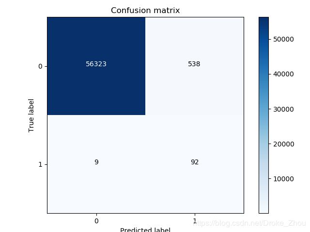
过采样的测试结果明显优于下采样的测试结果。

小结

采用下采样分析时，Recall值可以达到较高水平，但是误伤的概率较高，预测出的小概率事件发生量明显上升。采用过采样分析时，可以避免这个问题。