UCB中置信区间怎么推导出来的

Upper Confidence Bounds

Random exploration gives us an opportunity to try out options that we have not known much about. However, due to the randomness, it is possible we end up exploring a bad action which we have confirmed in the past (bad luck!). To avoid such inefficient exploration, one approach is to decrease the parameter ε in time and the other is to be optimistic about options with high uncertainty and thus to prefer actions for which we haven’t had a confident value estimation yet. Or in other words, we favor exploration of actions with a strong potential to have a optimal value.

The Upper Confidence Bounds (UCB) algorithm measures this potential by an upper confidence bound of the reward value, Û t(a)U^t(a), so that the true value is below with bound Q(a)≤Q̂ t(a)+Û t(a)Q(a)≤Q^t(a)+U^t(a) with high probability. The upper bound Û t(a)U^t(a) is a function of Nt(a)Nt(a); a larger number of trials Nt(a)Nt(a) should give us a smaller bound Û t(a)U^t(a).

In UCB algorithm, we always select the greediest action to maximize the upper confidence bound:

aUCBt=argmaxa∈Q̂ t(a)+Û t(a)atUCB=argmaxa∈AQ^t(a)+U^t(a)

Now, the question is how to estimate the upper confidence bound.

Hoeffding’s Inequality

If we do not want to assign any prior knowledge on how the distribution looks like, we can get help from “Hoeffding’s Inequality” — a theorem applicable to any bounded distribution.

Let X1,…,XtX1,…,Xt be i.i.d. (independent and identically distributed) random variables and they are all bounded by the interval [0, 1]. The sample mean is X⎯⎯⎯⎯t=1t∑tτ=1XτX¯t=1t∑τ=1tXτ. Then for u > 0, we have:

ℙ[[X]>X⎯⎯⎯⎯t+u]≤e−2tu2P[E[X]>X¯t+u]≤e−2tu2

Given one target action a, let us consider:

• rt(a)rt(a) as the random variables,
• Q(a)Q(a) as the true mean,
• Q̂ t(a)Q^t(a) as the sample mean,
• And uu as the upper confidence bound, u=Ut(a)u=Ut(a)

Then we have,

ℙ[Q(a)>Q̂ t(a)+Ut(a)]≤e−2tUt(a)2P[Q(a)>Q^t(a)+Ut(a)]≤e−2tUt(a)2

We want to pick a bound so that with high chances the true mean is blow the sample mean + the upper confidence bound. Thus e−2tUt(a)2e−2tUt(a)2 should be a small probability. Let’s say we are ok with a tiny threshold p:

e−2tUt(a)2=p Thus, Ut(a)=−logp2Nt(a)‾‾‾‾‾‾‾‾√e−2tUt(a)2=p Thus, Ut(a)=−log⁡p2Nt(a)

UCB1

One heuristic is to reduce the threshold p in time, as we want to make more confident bound estimation with more rewards observed. Set p=t−4p=t−4 we get UCB1 algorithm:

Ut(a)=2logtNt(a)‾‾‾‾‾‾‾√ and aUCB1t=argmaxa∈Q(a)+2logtNt(a)‾‾‾‾‾‾‾√Ut(a)=2log⁡tNt(a) and atUCB1=arg⁡maxa∈AQ(a)+2log⁡tNt(a)

Bayesian UCB

In UCB or UCB1 algorithm, we do not assume any prior on the reward distribution and therefore we have to rely on the Hoeffding’s Inequality for a very generalize estimation. If we are able to know the distribution upfront, we would be able to make better bound estimation.

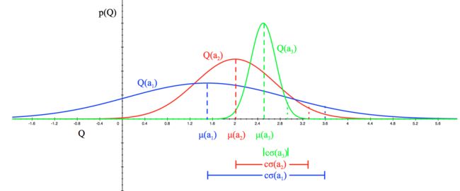
For example, if we expect the mean reward of every slot machine to be Gaussian as in Fig 2, we can set the upper bound as 95% confidence interval by setting Û t(a)U^t(a) to be twice the standard deviation.

Fig. 3. When the expected reward has a Gaussian distribution. σ(ai)σ(ai) is the standard deviation and cσ(ai)cσ(ai) is the upper confidence bound. The constant cc is a adjustable hyperparameter. (Image source: UCL RL course lecture 9’s slides)

Check my toy implementation of UCB1 and Bayesian UCB with Beta prior on θ.