基于tensorflow的线性回归
一、问题描述
我们使用俄勒冈州波特兰市的房价,其中X是房屋大小,Y是房价。该数据集包含47个示例。需要拟合Y与X的方程。
二、数据可视化
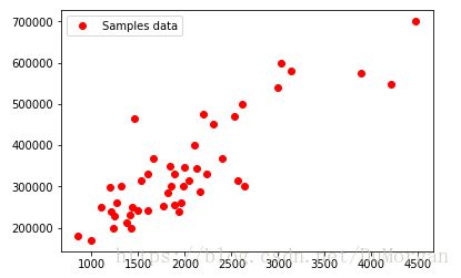
由图像可知,Y与X关系为一次线性方程。
三、算法实现
1、数据集预处理
规范化数据有助于提高梯度下降的性能,特别是在多元线性回归的情况下。
我们可以用下面的公式来做到这一点:
![]()
其中![]() 是变量的平均值,
是变量的平均值,![]() 是标准偏差。
是标准偏差。
实现代码:
def normalize(array):

return (array - array.mean()) / array.std()2、选择学习率
通常情况下,学习率是在如下范围内进行选择的:
![]()
对于这个任务,我们选择学习率为0.1。
3、实现成本函数并将梯度下降方法应用于最小化平方误差。
成本函数(cost_function)公式:
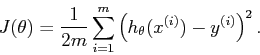
源代码中的实现:
cost_function = tf.reduce_sum(tf.pow(model - Y, 2))/(2 * samples_number)

optimizer = tf.train.GradientDescentOptimizer(learning_rate).minimize(cost_function)四、运行结果
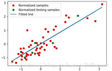
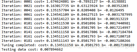
拟合出的直线比较精确,且成本函数值(cost)较小。
五、源代码
import tensorflow as tf
import numpy
import matplotlib.pyplot as plt

# Train a data set

size_data = numpy.asarray([ 2104,  1600,  2400,  1416,  3000,  1985,  1534,  1427,
  1380,  1494,  1940,  2000,  1890,  4478,  1268,  2300,
  1320,  1236,  2609,  3031,  1767,  1888,  1604,  1962,
  3890,  1100,  1458,  2526,  2200,  2637,  1839,  1000,
  2040,  3137,  1811,  1437,  1239,  2132,  4215,  2162,
  1664,  2238,  2567,  1200,   852,  1852,  1203 ])
price_data = numpy.asarray([ 399900,  329900,  369000,  232000,  539900,  299900,  314900,  198999,
  212000,  242500,  239999,  347000,  329999,  699900,  259900,  449900,
  299900,  199900,  499998,  599000,  252900,  255000,  242900,  259900,
  573900,  249900,  464500,  469000,  475000,  299900,  349900,  169900,
  314900,  579900,  285900,  249900,  229900,  345000,  549000,  287000,
  368500,  329900,  314000,  299000,  179900,  299900,  239500 ])


size_data_test = numpy.asarray([ 1600, 1494, 1236, 1100, 3137, 2238 ])
price_data_test = numpy.asarray([ 329900, 242500, 199900, 249900, 579900, 329900 ])

def normalize(array):
    return (array - array.mean()) / array.std()


size_data_n = normalize(size_data)
price_data_n = normalize(price_data)

size_data_test_n = normalize(size_data_test)
price_data_test_n = normalize(price_data_test)

plt.plot(size_data, price_data, 'ro', label='Samples data')
plt.legend()
plt.draw()
samples_number = price_data_n.size

X = tf.placeholder("float")
Y = tf.placeholder("float")

# Create a model
# Set model weights
W = tf.Variable(numpy.random.randn(), name="weight")
b = tf.Variable(numpy.random.randn(), name="bias")

learning_rate = 0.1
training_iteration = 200

model = tf.add(tf.multiply(X, W), b)

cost_function = tf.reduce_sum(tf.pow(model - Y, 2))/(2 * samples_number)
optimizer = tf.train.GradientDescentOptimizer(learning_rate).minimize(cost_function)

init = tf.initialize_all_variables()

with tf.Session() as sess:
    sess.run(init)
    display_step = 20
    # Fit all training data
    for iteration in range(training_iteration):
        for (x, y) in zip(size_data_n, price_data_n):
            sess.run(optimizer, feed_dict={X: x, Y: y})

        # Display logs per iteration step
        if iteration % display_step == 0:
            print( "Iteration:", '%04d' % (iteration + 1), "cost=", "{:.9f}".format(sess.run(cost_function, feed_dict={X:size_data_n, Y:price_data_n})),"W=", sess.run(W), "b=", sess.run(b))

    tuning_cost = sess.run(cost_function, feed_dict={X: normalize(size_data_n), Y: normalize(price_data_n)})
    print ("Tuning completed:", "cost=", "{:.9f}".format(tuning_cost), "W=", sess.run(W), "b=", sess.run(b))

    testing_cost = sess.run(cost_function, feed_dict={X: size_data_test_n, Y: price_data_test_n})
    print ("Testing data cost:" , testing_cost)

    plt.figure()
    plt.plot(size_data_n, price_data_n, 'ro', label='Normalized samples')
    plt.plot(size_data_test_n, price_data_test_n, 'go', label='Normalized testing samples')
    plt.plot(size_data_n, sess.run(W) * size_data_n + sess.run(b), label='Fitted line')
    plt.legend()
    plt.show()