Correlation and Regression
Sample Covariance
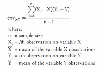
The covariance between two random variables is a statistical measure of the degree to which the two variables move together.
The covariance captures the linear relationship between two variables. A positive covariance indicates that the variables tend to move together; a negative covariance indicates that the variables tend to move in opposite directions.
The sample covariance is calculated as:
The actual value of the covariance is not very meaningful because its measurement is extremely sensitive to the scale of the two variables. Also, the covariance may range from negative to positive infinity, and it is presented in terms of squared units (e.g., percent squared when data are in percent). For these reasons, we take the additional step of calculating the correlation coefficient, which coverts the covariance into a standardized measure that is easier to interpret.
Sample Correlation Coefficient
The correlation coefficient, r, is a measure of the strength of the linear relationship (correlation) between two variables. The correlation coefficient has no unit of measurement; it is a "pure" measure of the tendency of two variables to move together.
The sample correlation coefficient for two variables, X and Y, is calculated as:
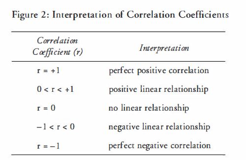
The correlation coefficient is bounded by positive and negative 1 (i.e., -1 <= r <= 1), where a correlation coefficient of +1 indicates that changes in the variables are perfectly positively correlated (i.e., they go up and down together, in lock-step). In contrast, if the correlation coefficient is -1, the changes in the variables are perfectly negatively correlated.
The interpretation of the possible correlation values is summarized in the following figure,
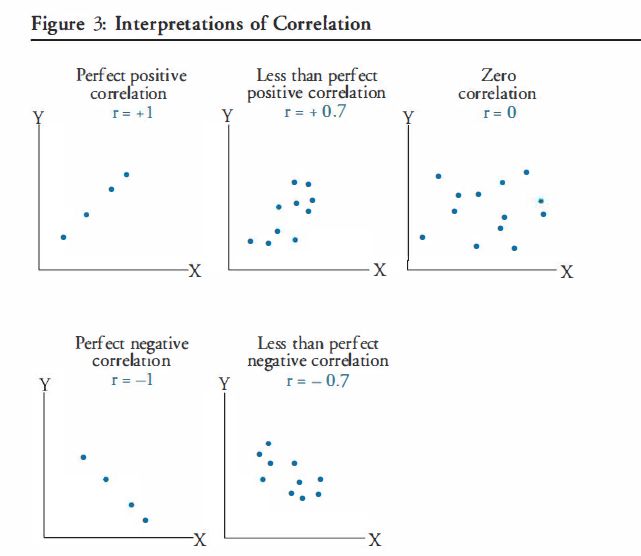
Interpreting a Scatter Plot
A scatter plot is a collection of points on a graph where each point represents the values of two variables(i.e. an X/Y pair).
Note that for r=1 and r=-1 the data points lie exactly on a line, but the slope of that line is not necessarily +1 or -1.
Limitations to Correlation Analysis
Outliers(异常值)
Outliers represent a few extreme values for sample observations. Relative to the rest of the sample data, the value of an outlier may be extraordinarily large or small. Outliers can result in apparent statistical evidence that a significant relationship exists when, in fact, there is none, or that there is no relationship when, in fact, there is a relationship.
Spurious Correlation (伪相关性)
Spurious correlation refers to the appearance of a causal linear relationship when, in fact, there is no relation. Certain data items may be highly correlated purely by chance.
Nonlinear Relationship
Correlation measures the linear relationship between two variables, it does not capture strong nonlinear relationships between variables.
Hypothesis testing the population correlation coefficient equals 0
The closer the correlation coefficient is to +1 or -1, the stronger the correlation. With the exception of these extremes(i.e. r=+/-1) we cannot really speak of the strength of the relationship indicated by the correlation coefficient without a statistical test of significance.
For our purpose, we want to test whether the correlation between the population of two variables is equal to zero.
Assuming that the two populations are normally distributed, we can use a t-test to determine whether the null hypothesis should be rejected. The test statistic is computed using the sample correlation, r, with n-2 degrees of freedom(df):
To make a decision, the calculated test statistic is compared with the critical t-value for the appropriate degrees of freedom and level of significance. Bearing in mind that we are conducting a two-tailed test, the decision rule can be stated as:
Simple Linear Regression(简单线性回归)
The purpose of simple linear regression is to explain the variation in a dependent variable in terms of the variation in a single independent variable. Here, the term "variation" is interpreted as the degree to which a variable differs from its mean value. Don't confuse variation with variance -- they are related but are not the same.
- The dependent variable is the variable whose variation is explained by the independent variable. The dependent variable is also referred to as the explained variable, the endogenous(内生的) variable or the predicated variable.
- The independent variable is the variable used to explain the variation of the dependent variable. The independent variable is also referred to as the explanatory variable, the exogenous(外生的) variable, or the predicating variable.
Assumption of Linear Regression
Linear regression requires a number of assumptions. As indicated in the following list, most of the major assumptions pertain to the regression model's residual term ε.
- A linear relation exists between the dependent and the independent variable.
- The independent variable is uncorrelated with the residuals.
- The expected value of the residual term is zero. [E(ε)=0]
The variance of the residual term is constant for all observations.

The residual term is independently distributed; that is, the residual for one observation is not correlated with that of another observation.

The residual term is normally distributed.
Simple Linear Regression Model
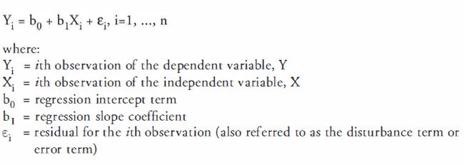
The following linear regression model is used to describe the relationship between two variables, X and Y:
Based on the regression model stated previously, the regression process estimates an equation for a line through a scatter plot of the data that "best" explains the observed values for Y in terms of the observed values for X.
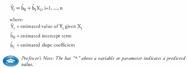
The linear equation, often called the line of the best fit, or regression line, takes the following form:
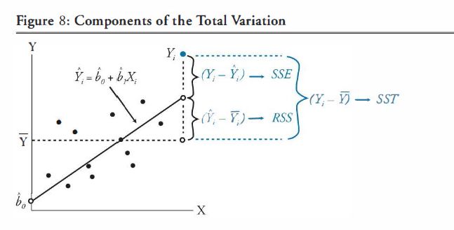
The regression line is just one of the many possible lines that can be drawn through the scatter plot of X and Y. In fact, the criteria used to estimate this line forms the very essence of linear regression. The regression line is the line for which the estimates of b0 and b1 are such that the sum of the squared differences (vertical distance) between the Y-values predicated by the regression equation and the actual Y-values is minimized. The sum of the squared vertical distances between the estimated and the actual Y-values is referred to as the sum of squared errors (SSE).
Thus, the regression line is the line that minimizes the SSE. This explains why simple linear regression is frequently referred to as ordinary least squares (OLS) regression, and the values estimated by the estimated regression equation are called least squares estimates.
The estimated slop coefficient for the regression line describes the change in Y for one unit change in X. It can be positive, negative, or zero, depending on the relationship between the regression variables. The slope term is calculated as:
The intercept term is the line's intersection with the Y-axis at X=0. It can be positive, negative, or zero. A property of the least squares method is that the intercept term may be expressed as:
The intercept equation highlights the fact that the regression line passes through a point with coordinates equal to the mean of the independent and dependent variables.
Keep in mind that any conclusion regarding the importance of an independent variable in explaining a dependent variable require determining the statistical significance of the slope coefficient. Simply looking at the magnitude of the slope coefficient does not address the issue of the importance of the variable. A hypothesis test must be conducted, or a confidence interval must be formed, to assess the importance of the variable.
SEE(Standard Error of Estimate)
The standard error of estimate(SEE) measures the degree of variability of the actual Y-values relative to the estimated Y-values from a regression equation. The SEE gauges the "fit" of the regression line. The smaller the standard error; the better the fit.
The SEE is the standard deviation of the error terms in the regression. As such, SEE is also referred to as the standard error of the residual, or standard error of the regression.
Coefficient of Determination (R^2) 决定系数
The coefficient of determination(R^2) is defined as the percentage of the total variation in the dependent variable explained by the independent variable. For example, an R^2 of 0.63 indicates that the variation of the independent variable explains 63% of the variation in the dependent variable.
For simple linear regression(i.e. one independent variable), the coefficient of determination, R^2, may be computed by simply squaring the correlation coefficient, r. In other words, R^2=r^2 for a regression with one independent variable. This approach is not appropriate when more then one independent variable is used in the regression.
Regression Coefficient Confidence Interval
Hypothesis testing for a regression coefficient may use the confidence interval for the coefficient being tested.
The confidence interval for the regression coefficient, b1, is calculated as:
In this expression, tc is the critical two-tailed t-value for the selected confidence level with the appropriate number of degrees of freedom, which is equal to the number of observations minus 2. (i.e. n-2)
The standard error of the regression coefficient is denoted as Sb1. It is a function of the SEE: as SEE raises, Sb1 also increases, and the confidence interval widens. This makes sense because SEE measures the variability of the data about the regression line, and the more variable the data, the less confidence there is in the regression model to estimate coefficient.
Hypothesis about a population value of a regression coefficient
A t-test may also be used to test the hypothesis that the true slope coefficient, b1, is equal to some hypothesized value. Letting b1^ be the point estimate for b1, the appropriate test statistic with n-2 degrees of freedom is:
The decision rule for tests of significance for regression coefficient is:
Rejection of the null means that the slope coefficient is different from the hypothesized value of b1.
To test whether an independent variable explains the variation in the dependent variable (i.e. it is statistically significant), the hypothesis that is tested is whether the true slope is zero (b1=0). The appropriate test structure for the null and alternative hypothesis is:
Confidence Interval for Predicated Values of the Dependent Variable
Confidence intervals for the predicated value of a dependent variable are calculated in a manner similar to the confidence interval for the regression coefficients.
The challenge with computing a confidence interval for a predicated value is calculating sf.
Analysis of Variance(ANOVA)
Analysis of variance(ANOVA) is a statistical procedure for analyzing the total variability of the dependent variable.
- Total sum of squares (SST) measures the total variation in the dependent variable. SST is equal to the sum of squared differences between the actual Y-values and the mean of Y:
Note: this is not the same as variance. Variance = SST/(n-1)
- Regression sum of square(RSS) measures the variation in the dependent variable that is explained by the independent variable. RSS is the sum of the squared distances between the predicated Y-values and the mean of Y.
- Sum of squared errors(SSE) measures the unexplained variation in the dependent variable. It's also known as the sum of squared residuals or the residual sum of squares. SSE is the sum of the squared vertical distances between the actual Y-values and the predicated Y-values on the regression line.
Thus, total variation = explained variation + unexplained variation, or:
SST = RSS + SSE The output of the ANOVA procedure is an ANOVA table, which is a summary of the variation in the dependent variable. ANOVA tables are included in the regression of output of many statistical software packages.
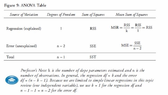
A generic ANOVA table for a simple linear regression(one independent variable) is presented in the following figure,
The mean regression sum of squares(MSR) and mean squared error(MSE) are simply calculated as the appropriate sum of squares divided by its degree of freedom.
Calculating R^2 and SEE
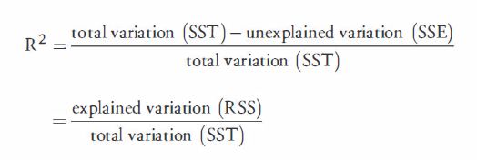
The R^2 and the standard error of estimate(SEE) can also be calculated directly from the ANOVA table. The R^2 is the percentage of the total variation in the dependent variable explained by the independent variable:
The SEE is the standard deviation of the regression error terms and is equal to the square root of the mean squared error (MSE):
Note: SSE is the sum of the squared residuals,, while SEE is the standard deviation of the residuals.
The F-Statistic
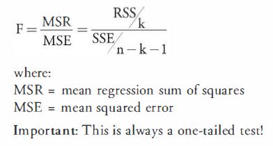
An F-test assesses how well a set of independent variables, as a group, explains the variation in the dependent variable. In multiple regression, the F-statistic is used to test whether at least one independent variable in a set of independent variables explains a significant portion of the variation of the dependent variable.
The F-statistic is calculated as:
In multiple regression, the F-statistic tests all independent variables as a group.
The F-Statistic With One Independent Variable
For simple linear regression, there is only one independent variable, so the F-statistic tests the same hypothesis as the t-test for statistical significant of the slope coefficient:
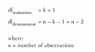
To determine whether b1 is statistically significant using the F-test, the calculated F-statistic is compared with the critical F-value, Fc, at the appropriate level of significance. The degrees of freedom for the numerator and the denominator with one independent variable are:
The decision rule for the F-test is:
Rejection of the null hypothesis as a stated level of significance indicates that the independent variable is significantly different than zero, which is interpreted to mean that it makes a significant contribution to the explanation of the dependent variable. In simple linear regression, it tells us the same thing as the t-test of the slope coefficient.In fact, in simple linear regression with one independent variable, F=tb1^2.
Limitations of Regression Analysis
Linear relationships can change over time. This means that the estimation equation based on data from a specific time period may not be relevant for forecasts or predictions in another time period. This is referred to as parameter instability.
Even if the regression model actually reflects the historical relationship between the two variables, its usefulness in investment analysis will be limited if other market participants are also aware of and act on this evidence.
If the assumptions underlying regression analysis do not hold, the interpretation and tests of hypotheses may not be valid.
